|
Copyright © 2008, Eli Lilly and Company and the National Institutes of Health Chemical Genomics Center. All Rights Reserved. For more information, please review the Privacy Policy and Site Usage and Agreement.
- IMMUNOASSAY DEVELOPMENT, OPTIMIZATION AND VALIDATION FLOW CHART
- INTRODUCTION
- IMMUNOASSAY PARAMETERS
- REAGENTS
- INSTRUMENTATION
- IMMUNOASSAY FORMATS
- IMPORTANT PARAMETERS FOR DEVELOPMENT OF AN IMMUNOASSAY
- INITIAL CONCEPT AND METHOD DEVELOPMENT OF A SANDWICH IMMUNOASSAY
- RESULTS
- INITIAL CONCEPT AND METHOD DEVELOPMENT OF A COMPETITIVE ASSAY
- DEVELOPMENT OF A COMPETITIVE IMMUNOASSAY
- METHOD VALIDATION (PRE-STUDY)
- METHOD VALIDATION (IN-STUDY)
- PRE-STUDY & IN-STUDY ACCEPTANCE CRITERIA
- REFERENCES
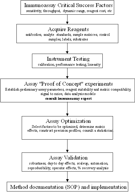
The intent of this document is to provide general guidelines to aid in the development, optimization and validation of an immunoassay. Following these guidelines will increase the likelihood of success in developing a robust immunoassay that will measure consistent values for unknown samples.
Immunoassays are used when an unknown concentration of an analyte within a sample needs to be quantified. To obtain the most accurate determination of the unknown concentration, an immunoassay must be developed based not only on the usual assay development criteria (SD window) but also on how well the immunoassay can predict the value of an unknown sample. First, one needs to establish the assay critical success factors. Then the immunoassay needs to be developed which establishes proof of concept. During the optimization phase the quantifiable range of the immunoassay method is determined by calculating a precision profile in the matrix in which the experimental samples will be measured. If the precision profile is within the desired working range, then assaying spiked recovery samples over several days completes the validation of the immunoassay. If the precision profile limits are not within the desired working range further optimization of the immunoassay is required prior to validation.
- Establish assay critical success factors.
- Ensure appropriate antibody and antigen reagents are available.
- Adsorb antigen or primary antibody to a solid surface.
- Block nonspecific binding sites to reduce background.
- Incubate the primary antibody with the sample.
- Wash off unbound reagents.
- Incubate secondary antibody-conjugate with sample.
- Wash off unbound reagents.
- Incubate substrate to generate signal.
- Calibration curve fitting, data analysis and quantitation by non-linear regression.
Immunoassays are used in screening to quantify the production or inhibition of antigens/haptens related to a disease target. These antigens or haptens are characteristic of the disease process, mediated by the target such as cytokines or growth factors. Hence the screening procedure will involve incubating compounds with specified target, usually expressed in cells, and collecting the cell medium or lysates to quantify the activity of the compounds. Several examples of this approach for using immunoassay procedures have been described in the literature (1-4). The critical steps in setting up a screen are as follows:
- Develop a validated immunoassay as described above.
- Acquire antibody, antigen/calibrator, label and buffer reagents in quantities needed for HTS.
- Establish liquid handling and automation procedures for screening and immunoassay methods.
- Establish stability of the primary capture antibody bound to a plate or antigen plate stability.
- Determine compound collections to be tested.
- Develop and validate a method for incubation of compounds with relevant target in the screening mode.
- Develop sample collection procedure from screening experiments.
- Develop data analysis procedures to use immunoassay data to derive compound potency such as IC50 or EC50.
It is important to establish a set of critical success factors before one begins the development, optimization and validation of an immunoassay:
- Analyte (hapten or antigen) to be measured.
- Sample matrices in which measurements will be made (serum, plasma, cell lysates, culture media etc.)
- Source of antibody, analyte standards and detection reagents (labeled antibody, enzyme substrates etc). Availability of these reagents is a critical requirement.
- Detection mode (colorimetric, fluorescence or chemiluminescence) and appropriate plate readers.
- Type of immunoassay to develop: Sandwich, competitive or antigen-down formats.
- Expected analyte concentration ranges to be measured: pg/ml, ng/ml or µg/ml in the sample matrix of choice. This would determine the detection limits and the measurable range that should be achieved in a validated assay.
- Data analysis models and format for reporting results.
- Validation and optimization criteria using statistical experimental design tools.
- Recovery, accuracy and precision expected at the limits of quantification and the measurable range.
- Sample throughput, frequency of use, automation and the number of laboratories that would run the assay.
- Control samples that would be used for optimization, validation and quality control runs.
Reagents are a critical piece of any assay development process. This refers to all of the reagents that will be used in the assay. There are certain items that need to be considered when obtaining reagents:
- Quality of standards and antibodies.
- Quantity of standards and antibodies.
- Purity of standards and antibodies (when possible antibodies are affinity purified).
- Selectivity and specificity of antibodies.
- Greiner high binding plates
- Costar EIA/RIA high-low binding plates
- Immunotech
- Falcon
Note: Other plate types can also be used based the experience of the investigators and appropriate quality control to demonstrate acceptability.
- 0.05 M sodium bicarbonate, pH 9.6
- 0.2 M sodium bicarbonate, pH 9.4
- PBS-50 mM Phosphate, pH 8.0, 0.15 M NaCl
- Carbonate-bicarbonate
- Phosphate Buffer: 1.7 mM NaH2PO4, 98 mM Na2HPO4.7H2O, 0.1% NaN3, pH 8.5
- TBS - 50 mM TRIS, pH 8.0, 0.15 M NaCl
- 1% BSA or 10% host serum in TBS, or TBS with 0.05% Tween-20
- Phosphate Buffer: 73 mM Sucrose, 1.7 mM NaH2PO4, 98 mM Na2HPO4.7H2Om 0.1% NaN3, pH 8.5
- 1% HSA in PBS
- Casein Buffer: Pierce Blocker cat # 37528
- Pierce has many blocking buffers that are available in their catalog
- PBS, 0.05% Tween-20, Chimeras
- TBS, 0.05% Tween-20, Chimeras
- 1% BSA or 10% host serum in TBS, or TBS with 0.05% Tween-20
- 1% BSA or 10% host serum in PBS, or PBS with 0.05% Tween-20
- 50 mM HEPES, 0.1 M NaCl, 1%BSA, pH 7.4
- Serum from the host animal-mouse serum, human serum, etc
- 0.1 M HEPES, 0.1 M NaCl, 1% BSA, 0.1 % Tween-20
- Tissue culture medium for samples.
- Cell lysates will contain SDS or other denaturing reagents that may interfere with the assay
- HRP: horseradish peroxidase
- TMB: 3,3', 5,5'-tetramethyl benzidine
- OPD: o-phenylene diamine
- ABTS: 2, 2'-azino-bis(3-ethylbenzthiazoline-6-sulfonic acid)
- HRP/TMB: 2M H2SO4 solution (at a 1:1 volume with the HRP/TMB substrate/enzyme solution)
- OPD: 3M H2SO4 solution, (at a 1:1 volume with the OPD substrate/enzyme solution)
- ABTS: 1%SDS
- HRP TMB: 450 nm
- OPD: 490 nm
- ABTS: 405 nm
- Sandwich Immunoassay: matched pair of antibodies, one for analyte capture on a solid surface and one for detection that binds to the antigen/hapten/analyte. Antibodies need to be affinity purified for optimal results.
- Competitive Immunoassay; a single antibody specific for the hapten/analyte. For optimal results affinity purified reagents are preferred.
- The analyte to be measured is typically a recombinant form of the natural analyte or peptide.
- Enough standard should be obtained for use in the development phase, validation phase and the continued support of the method to avoid changing lots and or running out of standard.
- Standard quality: Can vary from vendor to vendor and from lot to lot from a vendor.
- Standard stability: Information on the stability of a standard can be obtained from the vendor and their recommendations should be followed in storing the standards.
- Spiked controls are created by adding a known concentration of the standard analyte into the matrix (for example: tissue culture, serum, cell lysates). Spiked controls can be used to determine assay performance based on calculating the percent recovery.
- Control samples are real samples where the antigen analyte level has been determined by another validated method. Samples are aliquoted, frozen and used as control samples in each experiment to track assay performance.
The instrument used to read the output of the immunoassay should be tested initially for both linearity and performance. Instrument performance should be regularly calibrated according to manufacturer’s specifications. The majority of plate readers employ UV-Vis Absorbance, fluorescence or chemiluminescence signals as the measured response, since the products of enzyme labels are chromophores, fluorophores or emit luminescent signals. Linearity in response of the specific enzyme product of an ELISA should be checked at the appropriate wavelengths and instrument settings.
Lamp sources and Photomultiplier tubes (PMT) vary in quality and performance in many plate readers. The linear range of many plate readers is generally between 0-2.5 Absorbance units (AU), but other instruments have a linear range up to 4.0 AU. A malfunctioning lamp source or photomultiplier tube can significantly affect the linear response range.
These readers employ excitation and emission filter sets in addition to excitation lamp sources and photomultiplier tubes (PMT’s). In addition to the lamps and PMT’s, the filter sets also vary in quality, light throughput and bandwidth. Fluorescence signals are generally in Relative Fluorescence Units (RFUs) and linearity should be verified with appropriate filter sets for the fluorophores employed according to instrument specifications.
These instruments have sensitive photomultipliers to detect light emitted from a chemical reaction. No Lamp sources are necessary. These readers usually have a much larger dynamic range, thus allowing for the increase in sensitivity. Signals or responses are measured in Relative Light Units (RLU) and can be significantly different depending on their instrument design.
An enzyme-linked immunoassay (ELISA) is one of several methods used in the laboratory to detect and quantify specific molecules. ELISA’s rely on the inherent ability of an antibody to bind to the specific structure of a molecule. In order to optimize an ELISA and obtain the sensitivity and dynamic range required for the particular assay being developed, all the various components of the assay must be evaluated. The components will vary depending on the immunoassay format selected.
Following is a description of the various types of ELISA formats as well as reagents that needed to be optimized in order to obtain a robust assay.
Three frequently used types of ELISA are: sandwich assays, competitive assays and antigen down assays. The format selected depends on the reagents that are available and the dynamic range required for the particular assay. Sandwich assays tend to be more sensitive and robust and therefore tend to be the most commonly used.
A Sandwich Immunoassay is a method using two antibodies, which bind to different sites on the antigen or ligand. The primary antibody, which is highly specific for the antigen, is attached to a solid surface. The antigen is then added followed by addition of a second antibody referred to as the detection antibody. The detection antibody binds the antigen to a different epitope than the primary antibody. As a result the antigen is ‘sandwiched’ between the two antibodies. The antibody binding affinity for the antigen is usually the main determinant of immunoassay sensitivity. As the antigen concentration increases the amount of detection antibody increases leading to a higher measured response. The standard curve of a sandwich-binding assay has a positive slope. To quantify the extent of binding different reporters can be used. Typically an enzyme is attached to the secondary antibody which must be generated in a different species than primary antibodies (i.e. if the primary antibody is a rabbit antibody than the secondary antibody would be an anti-rabbit from goat, chicken, etc., but not rabbit). The substrate for the enzyme is added to the reaction that forms a colorimetric readout as the detection signal. The signal generated is proportional to the amount of target antigen present in the sample.
The antibody linked reporter used to measure the binding event determines the detection mode. For an ELISA, where the detection is colorimetric, a spectrophotometric plate reader is used. Several types of reporters have been recently developed in order to increase sensitivity in an immunoassay. For example, chemiluminescent substrates have been developed which further amplify the signal and can be read on a luminescent plate reader. Also, a fluorescent readout where the enzyme step of the assay is replaced with a fluorophor tagged antibody is becoming quite popular. This readout is then measured using a fluorescent plate reader.
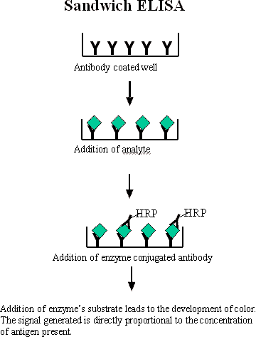
Figure 1
A competitive binding assay is based upon the competition of labeled and unlabeled ligand for a limited number of antibody binding sites. Competitive inhibition assays are often used to measure small analytes. These assays are also used when a matched pair of antibodies to the analyte does not exist. Only one antibody is used in a competitive binding ELISA. This is due to the steric hindrance that occurs if two antibodies would attempt to bind to a very small molecule. A fixed amount of labeled ligand (tracer) and a variable amount of unlabeled ligand are incubated with the antibody. According to law of mass action the amount of labeled ligand is a function of the total concentration of labeled and unlabeled ligand. As the concentration of unlabeled ligand is increased, less labeled ligand can bind to the antibody and the measured response decreases. Thus the lower the signal, the more unlabeled analyte there is in the sample. The standard curve of a competitive binding assay has a negative slope.
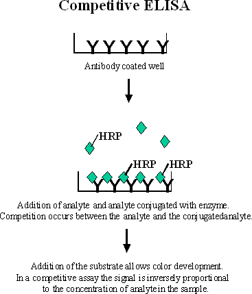
Figure 2
An antigen-down immunoassay or immunometric assay involves binding the antigen to a solid surface instead of an antibody. Antigen-down immunoassays are used to bind antibodies found in a sample. When the sample is added (such as human serum), the antibodies (IgE for example) from the sample bind to the antigen coated on the plate. A species-specific antibody (anti-human IgE for example) labeled with HRP is added next. The signal is directly proportional to the amount of antibody present in the sample; the more antibodies there are in the sample the higher the signal
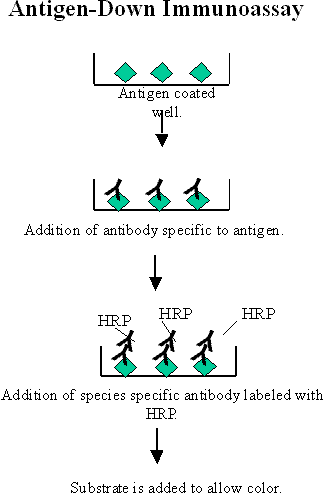
Figure 3
- Primary or capture antibody
- Secondary or detection antibody
- Plate type
- Coating buffer
- Blocking buffer/diluent buffer
- Wash buffer
- Coating antibody concentration
- Coated antibody stability
- Timing of each step in the immunoassay
- Secondary antibody concentration
- Reporter concentration
- Readout
- Instrument linearity
Goal: Develop a basic working method by determining the antibody which should be the primary/capture antibody and which antibody should be the secondary or detection antibody. Determine the optimum antibody concentrations for both the primary and secondary antibody.
Experiment: Coat the ELISA plate with several dilutions of both antibodies that will be used as part of the sandwich assay. Add the standard to be measured at a high, low and zero concentration. Use both of the antibodies at several concentrations as a secondary antibody. The results of this experiment will determine which antibody is best for both the capture antibody and the secondary antibody. The dilution needed for both antibodies will also be determined.
Reagents: Listed below is the plate type and buffers that will work for the majority of immunoassays. Use these buffers as a starting point.
- Two antibodies that recognize different epitopes on the analyte.
- A monoclonal for the capture and polyclonal for the detection antibody tend to yield the best sandwich assay.
- Greiner immunoassay plate.
- Coating buffer: 50mM sodium carbonate pH 9.6.
- Blocking buffer: 1% BSA, TBS, 0.1% Tween-20.
- Antibody diluent buffer: 1% BSA, PBS or TBS, 0.1 % Tween-20.
- Wash buffer: PBS or TBS, 0.1% Tween-20.
- TMB and HRP are used for enzyme/substrate readout.
- Acid stop buffer.
Protocol:
- Titrating both the primary capture antibody and the secondary detection antibody are made across a plate using a high, low and zero level of the analyte.
- Determine the desired working range of the analyte. This will give you the high and low concentrations.
- Dilute both antibodies in coating buffer at 0.5, 1 and 2 mg/ml and add 100 µl to each well of the 96-well microtiter plate.
- Incubate the plate containing the primary capture antibody overnight at 4°C then use the next day.
- Stability of the primary capture antibody bound to the plate can be determined in later experiments.
- Remove the primary capture antibody solution from the microtiter plates by aspirating or dumping the plate.
- Add 200 µl of blocking buffer to each well of the 96-well microtiter plate.
- Incubate the plate for one hour at RT.
- Remove the blocking buffer from the plate by aspirating or dumping the plate.
- Dilute the standard in dilution buffer to give a high and low concentration.
- Zero concentration will give you the NSB.
- Add 100 µl of the standard to each well in the microtiter plate and incubate for 2.5 hours at RT.
- Wash the plates 3 times with wash buffer.
- Dilute the secondary antibody serially at 1:200, 1:1000, 1:5000 and 1:25,000 in diluent.
- Add 100 µl of detection antibody to each well of the microtiter plate and incubate for 1 1/2 hours at RT.
- Wash the plates 3 times with wash buffer.
- Dilute streptavidin-HRP according to manufacture instructions in antibody diluent and add 100 µl to each well in the microtiter plate and incubate for 1 hr at RT.
- For HRP readout add either OPD or TMB as substrate to allow color development and incubate for 10-20 minutes at RT.
- Add acid stop reagent to stop the enzyme reaction.
- Read at 405 nm for TMB/HRP.
Plate Layout for Initial Experiment
Plate 1
|
Primary capture antibody A
|
|
Secondary Antibody
|
5 µg/ml
|
2 µg/ml
|
1 µg/ml
|
0.5 mg/ml
|
|
1:200
|
H
|
L
|
0
|
H
|
L
|
0
|
H
|
L
|
0
|
H
|
L
|
0
|
|
H
|
L
|
0
|
H
|
L
|
0
|
H
|
L
|
0
|
H
|
L
|
0
|
|
1:1000
|
H
|
L
|
0
|
H
|
L
|
0
|
H
|
L
|
0
|
H
|
L
|
0
|
|
H
|
L
|
0
|
H
|
L
|
0
|
H
|
L
|
0
|
H
|
L
|
0
|
|
1:5000
|
H
|
L
|
0
|
H
|
L
|
0
|
H
|
L
|
0
|
H
|
L
|
0
|
|
H
|
L
|
0
|
H
|
L
|
0
|
H
|
L
|
0
|
H
|
L
|
0
|
|
1:25000
|
H
|
L
|
0
|
H
|
L
|
0
|
H
|
L
|
0
|
H
|
L
|
0
|
|
H
|
L
|
0
|
H
|
L
|
0
|
H
|
L
|
0
|
H
|
L
|
0
|
Plate 2
|
Primary capture antibody B
|
|
Secondary Antibody
|
5 µg/ml
|
2 µg/ml
|
1 µg/ml
|
0.5 mg/ml
|
|
1:200
|
H
|
L
|
0
|
H
|
L
|
0
|
H
|
L
|
0
|
H
|
L
|
0
|
|
H
|
L
|
0
|
H
|
L
|
0
|
H
|
L
|
0
|
H
|
L
|
0
|
|
1:1000
|
H
|
L
|
0
|
H
|
L
|
0
|
H
|
L
|
0
|
H
|
L
|
0
|
|
H
|
L
|
0
|
H
|
L
|
0
|
H
|
L
|
0
|
H
|
L
|
0
|
|
1:5000
|
H
|
L
|
0
|
H
|
L
|
0
|
H
|
L
|
0
|
H
|
L
|
0
|
|
H
|
L
|
0
|
H
|
L
|
0
|
H
|
L
|
0
|
H
|
L
|
0
|
|
1:25000
|
H
|
L
|
0
|
H
|
L
|
0
|
H
|
L
|
0
|
H
|
L
|
0
|
|
H
|
L
|
0
|
H
|
L
|
0
|
H
|
L
|
0
|
H
|
L
|
0
|
Results:
H=High and L=Low: High ligand concentration in combination with the low ligand concentration will give an indication of the dynamic range.
L=Low: Low ligand concentration will give indication of sensitivity.
0=Zero: Zero ligand will give the non-specific binding (NSB) and indicate if there are background issues.
Determine the Absorbance units (A.U.) that yield the maximum signal to noise ratio or the greatest difference between the high and low analyte concentrations with the lowest variability. These are the conditions that will be selected for the antibody to be used as the primary capture antibody and the dilution of the antibodies to be used in the next experiment.
- If the background signal is unacceptably high (greater than 0.2 A.U.) then run additional experiments varying the plate type, blocking buffers, blocking buffers with a diluent agent like species specific IgG, antibody diluent buffers, wash buffers, and the reporter type.
- If the above general conditions have an acceptable NSB then determine if the dynamic range and sensitivity are in the appropriate range. To improve the sensitivity of the assay, the buffers, timing of incubations and matrix conditions can be varied in the next experiment.
- Antibodies are the reagents that play a major role in the sensitivity and dynamic range of an immunoassay. This is due to the actual antibody affinity for the analyte. If after attempting to develop the assay the sensitivity is still not in the desired range, different antibody pairs will need to be evaluated.
Example: An ELISA was set up to measure the amounts of an LP protein where there is only one polyclonal antibody available. The polyclonal antibody was used as both the primary capture antibody and the secondary detection antibody. Biotinylated antibody was used as the detection antibody.
Reagents:
- Pab- 0172B 140 µg/ml affinity pure antibody.
- LP276 230 µg/ml.
- LP276BT 400 µg/ml biotinylated affinity pure antibody.
Experiment: Follow the above protocol and plate layout
- Coated the affinity purified antibody at 3 levels: 2, 1 and 0.5 µg/ml
- Diluted the biotinylated antibody at 3 levels: 1:1000, 1:5000, and 1;25,000
- Diluted the standard LP276 protein in buffer to 50 ng/ml and 1 ng/ml
Plate Layout
|
Primary capture antibody
|
|
Secondary Antibody
|
2 µg/ml
|
1 µg/ml
|
0.5 µg/ml
|
|
1:1000
|
H
|
L
|
0
|
H
|
L
|
0
|
H
|
L
|
0
|
|
H
|
L
|
0
|
H
|
L
|
0
|
H
|
L
|
0
|
|
1:5000
|
H
|
L
|
0
|
H
|
L
|
0
|
H
|
L
|
0
|
|
H
|
L
|
0
|
H
|
L
|
0
|
H
|
L
|
0
|
|
1:25000
|
H
|
L
|
0
|
H
|
L
|
0
|
H
|
L
|
0
|
|
H
|
L
|
0
|
H
|
L
|
0
|
H
|
L
|
0
|
Average A.U. readings at A490
Actual results from initial experiment to determine the coating antibody and detection antibody
|
Primary capture antibody
|
|
Secondary Antibody
|
2 µg/ml
|
1 µg/ml
|
0.5 µg/ml
|
|
1:1000
|
3
|
1
|
1
|
3
|
1
|
1
|
3
|
1
|
1
|
|
4
|
1
|
1
|
4
|
1
|
1
|
3
|
1
|
1
|
|
1:5000
|
3
|
0.7
|
0.5
|
3
|
0.8
|
0.5
|
3
|
0.8
|
0.4
|
|
3
|
0.7
|
0.5
|
3
|
0.8
|
0.5
|
3
|
0.8
|
0.4
|
|
1:25000
|
1
|
0.2
|
0.1
|
1
|
0.2
|
0.1
|
1
|
0.3
|
0.1
|
|
1
|
0.2
|
0.1
|
1
|
0.3
|
0.1
|
2
|
0.3
|
0.1
|
Data summarized for the high, low and zero values for the LP276 protein concentration across the detection and primary antibody concentrations.
Values below are averages at an A.U. of A490.
LP 276 ng/ml
|
Secondary Antibody Conc.
|
50
|
1
|
0
|
50
|
1
|
0
|
50
|
1
|
0
|
|
1:1000
|
3.69
|
1.81
|
1.37
|
3.63
|
1.89
|
1.33
|
3.3
|
1.79
|
0.99
|
|
1:5000
|
3.22
|
0.7
|
0.49
|
3.24
|
0.81
|
0.47
|
3.1
|
0.83
|
0.36
|
|
1:25000
|
1.61
|
0.21
|
0.15
|
1.75
|
0.25
|
0.16
|
1.72
|
0.26
|
0.12
|
|
Primary Ab ug/ml
|
2
|
2
|
2
|
1
|
1
|
1
|
0.5
|
0.5
|
0.5
|
Conclusions: Lowest NSB and best signal to noise ratio from low to high LP276 concentration are the 0.5 µg/ml concentration for the coating antibody and the 1:25,000 dilution of the biotinylated antibody as the detection antibody.
Goal: To determine the matrix effect or sample type on the immunoassay method.
The matrix is based on what the sample is found in, for instance tissue culture media, serum, cell lysate, buffers, etc. Serum matrix, due to its complexity, can have a significant effect on the method. In this example the samples are in rat serum so the matrix effect of rat serum needs to be determined.
Experiment: The samples that need to be measured in this assay will be in either mouse or rat serum. Use the conditions established in the first experiment for the concentration of the primary capture antibody and the secondary detection antibody. Serially dilute the standard to obtain a full standard curve in 3 different matrices (10% rat serum, 30% rat serum and the original buffer diluent used in the first experiment). This will determine the matrix effect that will be used for the experimental samples.
Reagents:
- Use all of the reagents and buffers listed in the first experiment.
- Matrix diluent: 10% rat serum in antibody diluent or 30% rat serum in antibody diluent.
Protocol:
Follow the standard protocol changing only the matrix diluent to include rat serum.
- Dilute the primary antibody in coating buffer at 0.5 µg/ml and add 100 µl to each well of the 96-well microtiter plate.
- Incubate the plate containing the primary capture antibody overnight at 4°C and use the next day.
- Stability of the primary capture antibody bound to the plate can be determined in later experiments.
- Remove the primary capture antibody solution from the microtiter plates by aspirating or dumping the plate.
- Add 200 µl of blocking buffer to each well of the 96-well microtiter plate.
- Incubate the plate for one hour at RT.
- Remove the blocking buffer from the plate by aspirating or dumping the plate.
- Serially dilute the standard in antibody dilution buffer containing either 10% or 30% rat serum.
- Add 100 µl of the standard to each well in the microtiter plate and incubate for 2.5 hours at RT.
- Wash the plates 3 times with wash buffer.
- Dilute the detection antibody to 1:25,000 in antibody diluent.
- Add 100 µl of detection antibody diluent to each well of the microtiter plate and incubate for 1 1/2 hours at RT.
- Wash the plates 3 times with wash buffer.
- Dilute streptavidin-HRP according to manufacturer instructions in antibody diluent and add 100 µl to each well in the microtiter plate and incubate for 1 hr at RT.
- For HRP readout add either OPD or TMB as substrate to allow color development and incubate for 10-20 minutes at RT.
- Add acid stop reagent to stop the enzyme reaction.
- Read at 405 nm for TMB/HRP.
Results: Use the standard curve data and construct a precision profile. Check background levels. See page 138 for standard or calibration curve model fitting.
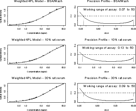
Note that the standard curves under all three matrix diluent conditions give the dynamic range and sensitivity necessary for the intended use. For this particular assay, there is no further development needed (based on the standard curve, low background and precision profile).
Precision Profile: Generate the precision profile for the standard curve of the appropriate matrix for the experiment. A web-based tool developed internally is available for computing the calibration curve and the precision profile that gives the estimated working range of the assay. The web address of this tool is http://pascal/statmath/calibration/prd/html/calibration.html.
A significant source of variability in the calibration curves can come from the choice of the statistical model used for the calibration curve. It is therefore extremely important to choose the correct calibration curve model. For most immunoassays, the models commonly available in software are the following.
Linear Model:
Response = a + b*(Concentration) + error,
where a and b are the intercept and slope respectively, and “response” refers to optical density or fluorescence reading from an immunoassay.
Quadratic Model:
Response = a + b*(Concentration) + c*(Concentration)2 + error,
where a, b and c are the intercept, linear and quadratic term coefficients respectively of this quadratic model.
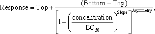
Four Parameter Logistic Model:

where the four parameters to be estimated are Top, Bottom, EC50 and Slope. Top refers to the top asymptote, Bottom refers to the bottom asymptote, and EC50 refers to the concentration at which the response is halfway between Top and Bottom.
Five Parameter Logistic Model:
Asymmetry is the fifth parameter in this model. It denotes the degree of asymmetry in the shape of the sigmoidal curve with respect to “EC50”. A value of 1 indicates perfect symmetry, which would then correspond to the four-parameter logistic model. However, note that the term referred to as “EC50” in this model is not truly the EC50. It is the EC50 when the asymmetry parameter equals 1. It will correspond to something very different such as EC20, EC30, EC80, etc., depending on the value of the asymmetry parameter for a particular data set. Further details are beyond the scope of this chapter.
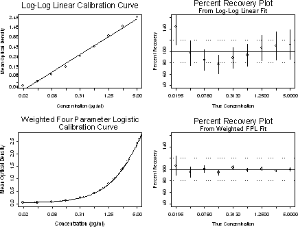
For most immunoassays, the four or five parameter logistic model is far better than the linear, quadratic or log-log linear models. These models have recently become available in several software packages, and are easy to implement even in an Excel-based program. As illustrated in the plots below, the quality of the model should be judged based on the dose-recovery scale instead of the lack-of-fit of the calibration curve (R2). In this illustration, even though the R2 of the log-log linear model is 0.99, when assessed in terms of the dose-recovery plot, this model turns out to be significantly inferior to the four parameter logistic model. Before the assay is ready for production, the best model for the calibration curve should be chosen based on the validation samples using dose-recovery plots.
The default curve-fitting method available in most software packages assigns equal weight to all the response values, which is appropriate only if the variability among the replicates is equal across the entire range of the response. However, for most immunoassays, the variability in the calibration-curve data between replicates increases proportionately with the response mean. Giving equal weight can lead to highly incorrect conclusions about the assay performance and will significantly affect the accuracy of results from the unknown samples. It is therefore extremely important to use a curve-fitting method/software that has appropriate weighting methods/options. See Appendix for more details.
The two-step experiment detailed above is a very simple example of how to develop a sandwich ELISA method. If the dynamic range and sensitivity of the assay does not meet the needs of the experiments then further experimental conditions should be tested using experimental design. With experimental design all of the factors involved in the ELISA including buffers, incubation time and plate type can be analyzed.
In a sandwich ELISA method the antibodies chosen are the major drivers of the assay parameters. If at this point in the method development the precision profile of the standard curve is extremely far from the desired dynamic range and sensitivity, instead of continuing with development experiment, antibodies should be further characterized. Changing some of the variables such as the Ab concentrations can significantly improve the calibration curve and hence it’s precision profile.
Goal: Determine the optimal conditions for the variables in the immunoassay including incubation steps, buffers, substrate, etc. Also, determine the optimal antibody concentrations and the stability of the primary capture antibody bound to the plate.
Experiment: Dilute the standard in the matrix compatible to the sample (as determined in the second experiment). Vary the incubation times, dilution buffers and other variables in order to optimize the immunoassay. Analyze by using experimental design software and precision profiles.
Reagents:
- Coating buffers
- Blocking buffers
- Wash buffers
- Antibody diluents
- Substrate
Protocol:
- Coat the microtiter plate with the primary capture antibody at the concentration determined in the initial experiment. Incubate overnight at 4°C.
- Discard the primary capture antibody solution from the microtiter plate.
- Block the plate for 1 hour at RT using various blocking reagents.
- Store plates at 4°C, desiccated, for several periods of time 0-5 days.
- Repeat steps 1-3 the day of the actual experiment.
- Serially dilute, using an 8-point standard curve, the known standard in the appropriate matrix for the experiment. For the control also dilute the standard in the same buffer as was used in the initial experiment. Add 100 µl of standard to each well in the 96-well microtiter plate.
- Incubate the diluted standard with the primary capture antibody for 1 hour and 3 hours at RT and overnight at 4°C. Each time point will have to be run in a separate plate.
- Wash plates 3 times (If background or NSB is high try different wash buffers).
- Add 100 µl of diluted secondary detection antibody. If background is high again different diluents can be tested.
- Incubate the secondary detection antibody for different time periods and again different plates will have to be used for each time condition.
- Wash plates 3 times.
- Add 100 µl of substrate to the plate containing the detection antibody conjugated to the enzyme and allow to incubate according to the manufacturers conditions.
- Add 100 µl of stop buffer.
- Read at 405 nm.
Data Analysis: Compute the standard curves and their precision profiles for all the experimental design conditions. Derive the optimization endpoints using the precision profiles. Then analyze the optimization endpoints using software such as JMP to determine the optimum levels of the assay factors. See next section for the details and illustration.
Step 1:
Identify all the factors/variables that potentially contribute to assay sensitivity and variability. Choose appropriate levels for all the factors (high and low values for quantitative factors, different categories for qualitative factors). Then use fractional-factorial experimental design in software such as JMP to derive appropriate experimental “trials” (combinations of levels of all the assay factors). Run 8-point calibration curves in duplicate for each trial. With each trial taking up two columns in a 96-well plate 6 trials per plate can be tested. All trials should be randomly assigned to different pairs of columns in the 96-well plates. However, certain factors such as incubation time and temperature are inter-plate factors. Therefore, levels of such factors will have to be tested in separate plates.
|
|
Trial 1
|
Trial 2
|
Trial 3
|
Trial 4
|
Trial 5
|
Trial 6
|
|
1
|
2
|
3
|
4
|
5
|
6
|
7
|
8
|
9
|
10
|
11
|
12
|
|
A
|
8pt. calibration curve; duplicate
|
8pt. calibration curve; duplicate
|
8pt. calibration curve; duplicate
|
8pt. calibration curve; duplicate
|
8pt. calibration curve; duplicate
|
8pt. calibration curve; duplicate
|
|
B
|
|
|
|
|
|
|
|
|
|
|
|
|
|
C
|
|
|
|
|
|
|
|
|
|
|
|
|
|
D
|
|
|
|
|
|
|
|
|
|
|
|
|
|
E
|
|
|
|
|
|
|
|
|
|
|
|
|
|
F
|
|
|
|
|
|
|
|
|
|
|
|
|
|
G
|
|
|
|
|
|
|
|
|
|
|
|
|
|
H
|
|
|
|
|
|
|
|
|
|
|
|
|
After the above experiment is run the calibration curves should be fit for each trial using an appropriately weighted-nonlinear regression model. Then the precision profile for the calibration curve of each trial should be obtained along with the important optimization end-points such as working-range, lower quantitation limit and precision area. Now analyze these data to determine the optimal level of all qualitative factors and determine which factors should be further investigated. See Appendix for the definition of these terms/concepts and details on the computations.
Step 2:
We now need to determine the optimum levels for the factors determined in the previous step. Choose appropriate low, middle and high levels for each of these factors based on the data analysis results from step 1. Now use software such as JMP to generate appropriate trials (combinations of low, middle and high levels of all the factors) from a central-composite design. Then run duplicate 8-point calibration curves for each trial using a similar plate format as in step 1.
Now obtain the precision profile and the relevant optimization end-points of the calibration curve of each trial. Perform the response-surface analysis of these data to determine the optimal setting of each of the quantitative factors run in this experiment.
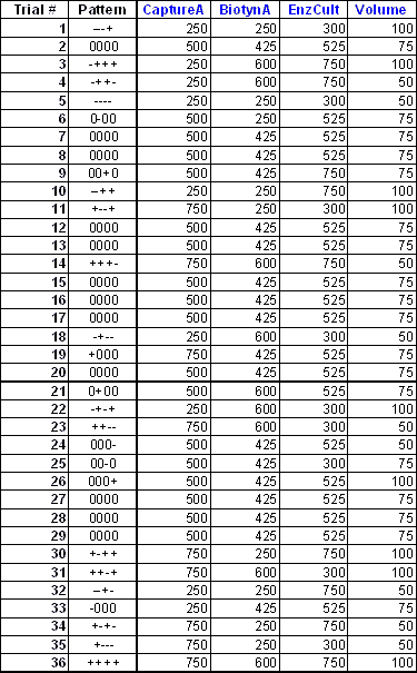
In this table, we have the experiment plan from the second step of the optimization process using experimental design for a sandwich ELISA. These four factors (primary capture antibody, secondary detection antibody, enzyme and volume) were picked out of the six factors considered in the first step of this optimization process (screening phase) for further optimization. We use a statistical experimental design method called central composite design to generate the appropriate combinations of the high, mid and low levels of the four factors in this second step. For example, trial #6 in this table refers to the middle level of the first, third and the fourth factors, and the low level of the second factor.
8-point standard curves in duplicate were generated for each of these trials, in adjacent columns of a 96-well plate. This resulted in six trials per plate, and with 36 trials in 6 plates.
We computed the precision profiles of the calibration curves of each of these 36 trials. From these precision profiles, we computed the working range (lower and upper quantification limits), CV and related variability and sensitivity measures. We then used a statistical data analysis method called "response surface analysis" on these summary measures. This resulted in polynomial type models for all the factors. Using the shape of the curve and other features from this model, the optimum levels for these factors were determined. This gave us the most sensitive dynamic working range possible for this assay.
An experiment was then performed for this ELISA to compare these optimized levels to the pre-optimum levels and the assay kit manufacturer’s recommendation. The results from this comparison are summarized below.
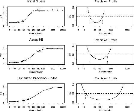
The optimized levels derived from statistical experimental design for this ELISA resulted in the following improvements over the pre-optimum and assay kit manufacturer’s recommendation.
- Lower quantification limit decreased more than two-fold to 13.6 nM.
- Upper quantification limit by up to 10-fold to 1662.3 nM.
- Precision area increased by 2-fold and the working range increased by 2-fold to two log cycles.
This improvement is evident from the precision profiles given above for these three conditions.
Development and validation of a competition immunoassay requires considerable expertise in reagent characterization and method development. Sandwich and antigen-down immunoassays formats should be explored before attempting the competitive immunoassay format.
- A competitive immunoassay is not as sensitive as a sandwich ELISA.
- A competitive immunoassay is more sensitive to matrix issues, especially serum matrix, which can affect assay performance.
- Timing of the various incubation steps is less robust in a competitive assay. That is the IC50 of the standard curve will shift with minor changes in incubation of the various steps of the immunoassay.
- The labeling of the hapten or analyte can change the analyte binding affinity for the antibody. Experiments need to determine the effect of the label on the binding affinity of the antibody to the analyte.
Goal: Determine the optimal coating concentration of the antibody used for capture and the labeled ligand.
Reagents:
- Antibody- mono or polyclonal, specific to the analyte.
- Buffers- same as for a competitive assay.
- Labeled ligand-the enzyme or biotin is labeled directly to the analyte or ligand.
Experiment: Coat the ELISA plate with various antibody concentrations to determine the optimal concentration of antibody and labeled ligand.
Protocol:
- Determine the desired analyte working range.
- Titrate capture antibody using high, low and zero analyte concentration levels.
- Dilute the capture antibody in coating buffer at 0.1, 0.5, 1 and 2 mg/ml and add 100 µl to each well of the 96-well microtiter plate. The capture antibody may need to be titrated down further. The amount of antibody coated on the plate will be proportional to the sensitivity of the assay.
- Incubate the plate containing the primary capture antibody overnight at 4°C and use the next day.
- Stability of the primary capture antibody bound to the plate can be determined in later experiments.
- Remove the primary coating antibody solution from the microtiter plates by aspirating or dumping the plate.
- Add 200 µl of blocking buffer to each well of the 96-well microtiter plate.
- Incubate the plate for one hour at RT.
- Remove the blocking buffer from the plate by aspirating or dumping the plate.
- Dilute the labeled standard in antibody dilution buffer over a wide range. The desired result is the condition, which gives a readable signal with the least amount of antibody coated, in combination with the least amount of labeled standard.
- Zero concentration will give you the NSB.
- Add 100 µl of the labeled standard to each well in the microtiter plate and incubate for 2.5 hours at RT. (The standard can either be directly labeled with the enzyme or biotinylated).
- Wash the plates 3 times with wash buffer.
- If a biotinylated standard is used, Dilute streptavidin-HRP according to manufacturer’s instructions in antibody diluent and add 100 µl to each well in the microtiter plate and incubate for 1 hr at RT.
- For HRP readout add either OPD or TMB as substrate to allow color development and incubate for 10-20 minutes at RT.
- Add acid stop reagent to stop the enzyme reaction.
- Read at 405 nm for TMB/HRP.
- Determine the linearity of the instrument being used for the readout the same way as described for a sandwich ELISA.
Goal: Determine the potential dynamic range and sensitivity. Take the conditions established in the initial experiment for the concentration of the antibody and labeled ligand and incubate with a wide range of unlabeled analyte. The resulting standard curve and precision profile calculation will give an estimate of the sensitivity and dynamic range of the assay.
Reagents: Reagents are the same as in initial experiment.
Protocol:
- Dilute the capture antibody in coating buffer at the concentration determined in the initial experiment. Add 100 µl to each well of the 96-well microtiter plate.
- Incubate the plate containing the primary capture antibody overnight at 4°C and use the next day.
- Remove the primary capture antibody solution from the microtiter plates by aspirating or dumping the plate.
- Add 200 µl of blocking buffer to each well of the 96-well microtiter plate.
- Incubate the plate for one hour at RT.
- Remove the blocking buffer from the plate by aspirating or dumping the plate.
- Dilute the labeled standard in antibody dilution buffer at the concentration determined in the initial experiment.
- Dilute the unlabeled ligand in antibody dilution buffer over a wide range of concentrations.
- Add 100 µl of the labeled standard to each well in the microtiter plate and 100 µl of the various dilution of the unlabeled ligand. Incubate for 2.5 hours at RT. This is the competitive part of the assay and will allow for the competition between the labeled and unlabeled ligand to compete for the sites on the antibody.
- Wash the plates 3 times with wash buffer.
- If a biotinylated standard is used, Dilute streptavidin-HRP according to manufacturer’s instructions in antibody diluent and add 100 µl to each well in the microtiter plate and incubate for 1 hr at RT.
- For HRP readout add either OPD or TMB as substrate to allow color development and incubate for 10-20 minutes at RT.
- Add acid stop reagent to stop the enzyme reaction.
- Read at 405 nm for TMB/HRP.
Goal: Determine the optimal buffers, incubation periods, temperatures, matrix effects, and other variables that may affect the assay.
Reagents: Reagents are the same as in initial experiment.
Protocol: Same as in previous experiment except for the following changes at steps 8 and 9:
- Dilute the unlabeled ligand in antibody dilution buffer, and the matrix appropriate for the experiment, over a wide range of concentrations. Again the dilution buffer can be varied here according to the experimental design.
- Add 100 µl of the labeled standard to each well in the microtiter plate and 100 µl of the various dilution of the unlabeled ligand. Incubate for 2.5 hours at RT. This incubation time can be varied for longer and shorter periods of time to potentially increase the sensitivity and dynamic range of the assay.
Results: Analysis of the results is by use of JMP or other appropriate statistical software to determine the optimal conditions for incubation timing, buffers for dilution, and matrix effects.
It is important to note that the precision profile is based on just the calibration curve. Consequently only the calibration curve factors (quality and stability of reference standards, quality and stability of reagents, statistical validity of the calibration curve model) are taken into account for deriving these quantitation limits. Sample factors such as analyte (similar physicochemical substances), matrix (other substances that can affect analytical result) and operational factors can affect the performance of the assay/method as well. Thus the quantitation limits derived from the precision profile of a calibration curve is an optimistic assessment of method performance. If these limits are not satisfactory, we need to re-optimize the assay further.
If the quantitation limits from the precision profile are close to the limits desired for the method’s intended use, proceed to a full validation experiment as outlined below. This validation experiment is used to establish the method quantitation limits using the analysis of recovery data from validation samples (spiked standards). This experiment will take into account the three major sources of variation described above (calibration curve factors, sample factors and operational factors).
For the full validation experiment, generate the following data in at least three independent runs.
- Calibration curve in each run, preferably in triplicate.
- Validation/QC samples (independent set of samples spiked with known amount of standards) in each run at six concentrations with four replicates; three concentrations near the precision profile estimates of lower and upper quantification limits, and three more equally spaced between lower and upper quantification limits.
- Estimate the concentrations of the validation samples of each run using the respective calibration curves. Then compute the % recovery of these validation samples using the following formula:
% Recovery = 100*(Estimated Concentration)/True Concentration
- Now compute the average and standard error of the % recovery data of the validation samples from all runs for each concentration. Then standard error should be based on a separate variance component analysis of the multiple runs of validation data, and it should include the sources of variability relevant during the use of the assay in production. At the minimum, it will include inter-run and intra-run variability. Some of the other sources to consider may be analyst, plate, equipment, etc.
- Plot the average % recovery values along with the standard error (as calculated above) versus the true concentrations. Note that the % recovery along with the standard error as determine above reflects the Total Error of the assay.
- The %recovery and the standard error limits must be within +/- X% of the nominal value. If X is 30 of the nominal value at each concentration (i.e., 70% to 130%). That is, this means that the Total Error of the assay must be within 30%. The value of X should be set based on the intended use of the assay. Recommendations on the acceptance criteria are discussed later in this chapter.
- If X is set at 30%, the lower quantification limit is the lowest concentration at which the % recovery is within 70% to 130%. The upper quantification limit is the highest concentration at which the % recovery is within 70% to 130%.
The in-study validation phase is about making sure that the assay continues to perform per pre-defined specifications in each study run. During production phase, when the assays are being used for screening the unknowns, it is important to run validation/QC samples in every run with at least 2 replicates at high, middle and low concentrations (just one or two columns of a 96-well plate). Compute the average % recovery of these samples to make sure that the average recovery is within a reasonable range of accuracy (say, 80% to 120%). This might be adequate for quality control and is a reasonable compromise for any loss in assay throughput. Various methods may be considered for setting criteria for accepting or rejecting a study run during production run (in-study validation). This is addressed in a subsequent section in this chapter.
Set up numerous aliquots of the standard and store frozen at –70°C. If the standard concentration is much higher than the first point on your curve, pre-dilute it so that a single, simple dilution can be made in order to set up the standard curve.
Dilute the standards serially to obtain an 8 point standard curve in the matrix appropriate for the samples that need to be measured. For example if measuring tissue culture samples then the standards should be diluted in the same tissue culture medium that the samples are in. For serum samples, the standards should be diluted in serum diluted with an optimized buffer to the same dilution that the samples will be diluted.
Set up a series of spiked samples, again in the matrix appropriate for the samples that will be measured. The spiked control samples should not be the same concentration as in the standard curve and should cover the detectable range that the samples are thought to cover.
Follow the immunoassay protocol established during the optimization experiments. Set up the plate with 3-4 replicates of the standard curve and 4 or more replicates of the spiked control samples.
Assay at least 3 plates over 3 different days for a complete validation.
|
St1
|
St1
|
St1
|
St1
|
SP1
|
SP1
|
SP1
|
SP1
|
|
St2
|
St2
|
St2
|
St2
|
SP2
|
SP2
|
SP2
|
SP2
|
|
St3
|
St3
|
St3
|
St3
|
SP3
|
SP3
|
SP3
|
SP3
|
|
St4
|
St4
|
St4
|
St4
|
SP4
|
SP4
|
SP4
|
SP4
|
|
St5
|
St5
|
St5
|
St5
|
SP5
|
SP5
|
SP5
|
SP5
|
|
St6
|
St6
|
St6
|
St6
|
SP6
|
SP6
|
SP6
|
SP6
|
|
St7
|
St7
|
St7
|
St7
|
SP7
|
SP7
|
SP7
|
SP7
|
|
St8
|
St8
|
St8
|
St8
|
SP8
|
SP8
|
SP8
|
SP8
|
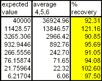
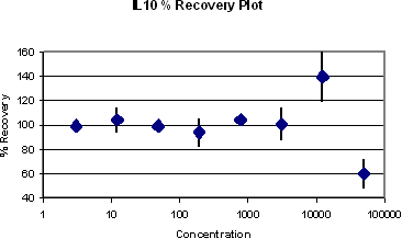
The %recovery and the standard error that takes into account of the relevant sources of variation are plotted below. If X is 30%, then the quantification limits are the lowest and highest concentrations where the %recovery are within 70% to 130%. So for this assay, the lower quantification limit is the lowest concentration tested in this validation study (6.2 pg/ml), and the upper quantification limit is 3265 pg/ml.
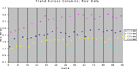
IL-10
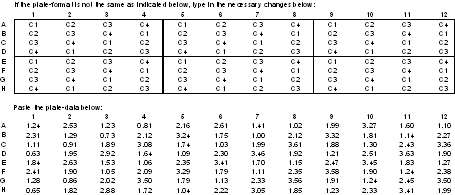
It is important to check whether there is any systematic data trend across rows or columns of the 96-well plate and whether there is any significant variability between plates. An experiment with three plates and four concentrations of the standard can be done using the plate-layout given below. In this layout, C1, C2, C3 and C4 denote the standard concentrations from lowest to highest. For the purpose of illustration, data from one of the plates and a plot of the data from this experiment are given below for a sandwich ELISA. A systematic trend across columns is evident from this plot. For determining the statistical significance of this trend and the plate to plate variability, further statistical analysis of the data can be done with the help of a statistician.
Different methods of quality control are available and routinely used in analytical methods. It is important that the methods used for assessment of method performance are suitable for the intended purpose.
The use of QC methods used in PK assays (eg 4-6-x) and clinical diagnostics (confidence limits) may both be applicable. It is up to the laboratory performing the analysis to choose the most relevant method to use and justify it scientifically based on statistical and clinical criteria. This will be critical when using 4-6-x in order to assign an appropriate value to ‘x’.
Shah et al (1990) proposed the 4-6-X rule for in-study validation phase that has become popular and widely used. This rule states that 4 out of the total 6 samples should be within X% of the nominal/reference value, and at least one out of the two samples at each level must be within X% of the reference value. The choice of X is specified a priori based on the intended use and purpose of the assay, and it was set at 20% by Shah et al. DeSilva et al (2003) proposed the following criteria for pre-study and in-study validation phase of ligand-binding assays for assessing pharmacokinetics of macromolecules.
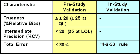
It should be noted that the acceptance criteria for biomarker assays will depend heavily on the intended use of the assay and should ideally be based on physiological variability as well. According to the criteria listed in this table, X is set at 30% for in-study validation, and the total error is set to be within 30% for the pre-study validation, along with the 20% limits for each component of total error (bias and precision). The pre-study criteria (Total Error < X%) and the in-study criteria (4-6-X rule) are not entirely consistent because it does not take into account total error estimate variability and the consequent decision error rates. Thus the uncertainty in these estimates will depend on the magnitude of the errors and the number of measurements, and will in turn impact the level of decision error rates (Kringle, 1994). The appropriate value of X in 4-6-X can be determined based on the variability of the total error estimates in pre-study validation. When it is feasible to use more QC samples in each run, 8-12-X or 10-15-X will have much better statistical outcomes than the 4-6-X criteria. In addition, the use of control charts as described by Westgard or tolerance limits based on pre-study validation data may be considered when possible.
The concept of total error as the primary parameter, and with bias and precision as additional constraints is very useful. This is because total error has a more practical and intuitive appeal as it relates specifically to our primary question of interest about the assay; How far are my observed test results from the reference/nominal value? Since this is the primary practical question in the minds of most laboratory scientists, the criteria on the assay performance for the in-study phase is defined with respect to this question. Therefore the primary criteria for the pre-study phase are also defined with respect to this question, that is, the total error.
Given that this total error approach is very intuitive and practical, it is important to consider a rule that will provide better consistency between our expected performance for the assay to the in-study and pre-study validation criteria.
Consideration of Physiological Variation for Acceptance Criteria:
One of the most important considerations for defining the performance criteria of most biomarker methods is the physiological variability in the study population of interest. That is, in order to determine whether a biomarker method is ‘fit-for-purpose’, we should determine whether it is capable of distinguishing changes that are statistically significant based on the intra-subject and inter-subject variation. The term “subject” here may refer to animal or human. For example, an assay with 50% total error during pre-study validation may still be adequate for detecting a 2-fold treatment in a clinical trial for a certain acceptable sample size. Thus whenever possible, the acceptance criteria for pre-study validation should be based on physiological variation in the study. An example of the use of intra-subject and inter-subject variation for defining the pre-study acceptance criteria can be found in http://www.westgard.com/guest17.htm.
When the relevant physiological data (say, treated patients of interest) are not available during the assay validation phase, then healthy donor samples should be used to estimate the intra and inter subject variation, and hence the desired specifications on the pre-study assay validation. This can be updated at a later time when there is access to the relevant patient data. If access to healthy donor samples is also not feasible, then other flexible biological rationale should be considered and updated periodically as more information become available over time. In the absence of physiological data or other biological rationale, the acceptance criteria for pre-study validation should not be strictly defined. Instead, only the performance characteristics from pre-study validation such as the bias, precision and total error should be reported. Any decision regarding the acceptance of the assay (pre-study acceptance criteria) and consequently the determination of the dynamic range (LQL, UQL) should be put on hold until adequate information related to the physiological data become available.
Assessment of analytical batches/runs in terms of acceptance (in-study validation) needs to take into account of the study need. Setting critical acceptance criteria a priori may not be appropriate (or even possible) to take into account all possible outcomes in the analytical phase – especially since the values seen in the incurred samples may not be what is expected or predicted. This is especially the case in new or novel BM’s as opposed to those where historical information in normal and diseased populations is available.
It is advised that when constructing batches for analysis, ALL levels of QC’s are analyzed at each QC interval. For example, a batch of 96-well microtiter plates may include 3 sets of QC’s at start, middle and end of the plate, and all QC’s (Low,Medium,High) are assayed at all three intervals. This will help in the assessment of method performance and batch acceptance for incurred samples.
In studies with large numbers of samples, assessment of method performance between batches may help before rejecting data. For example, it is of no value to reject batches when large numbers of high concentration QC’s fail but where the low and medium QC’s are good AND when all the study sample results are in the low to medium range. Here the positioning of the high QC based on expectation before the analysis of incurred samples has been flawed – but it does not necessarily make the study sample results.
Swartzman EE, Miraglia SJ, Mellentin-Mitchelotti J, Evangelista L, Pau-Miay Y, “A Homogeneous Multiplexed Immunoassay for High-Throughput Screening Using Fluorometric Microvolume Assay Technology”, 1999, Analytical Biochemistry, 271, 143-151.
Stockwell BR, Haggarty SJ, Schreiber SL, High-Throughput Screening of Small Molecules in Miniaturized Mammalian Cell—Based Assays Involving Post-translational Modifications”, 1999, Chemistry & Biology, 6, 71-83.
Martens C, Bakker A, Rodriguez A, Mortensen RB, Barrett RW, “A Generic Particle-Based Nonradioactive Homogeneous Multiplex Method for High-Throughput Screening Using Microvolume Fluorimetry”, 1999), Analytical Biochemistry, 273, 20-31.
Zuck P, Lao Z, Skwish S, Glickman JF, Yang K, Burbaum J, Inglese J, “ Ligand-receptor binding measured by laser scanning imaging”, 1999, PNAS, 96, 11122-11127.
Web sites
- http://www.brendan.com/
- http://www.waichung.demon.co.uk/webanim/Menu1.htm
|