|
July 19, 2005
| Region | Season | Predicted Mean Number of Illnesses per Annuma | |||
|---|---|---|---|---|---|
| Baseline | Immediate Refrigeration (~1 log10 Reduction) | 2-log10 Reduction | 4.5-log10 Reduction | ||
| Gulf Coast Louisiana | Spring | 505 (36, 1.6x10³) | 54 (3.0, 180) | 5.2 (0.35, 17) | 0.017 (1.1x10⁻³, 0.053) |
| Summer | 1,406 (109, 4.4x10³) | 139 (7.6, 490) | 15 (1.1, 47) | 0.046 (3.5x10⁻³, 0.15) | |
| Fall | 132 (6.4, 470) | 8.8 (0.34, 34) | 1.3 (0.060, 5.0) | 4.2x10⁻³ (2.0x10⁻⁴, 0.016) | |
| Winter | 6.7 (0.16, 26) | 0.80 (0.04, 2.5) | 0.070 (1.7x10⁻³, 0.30) | 2.2x10⁻⁴ (3.9x10⁻⁶, 9.8x10⁻⁴) | |
| Gulf Coast (Non-Louisiana) | Spring | 193 (13, 630) | 29 (1.5, 98) | 2.0 (0.13, 6.3) | 6.2x10⁻³ (4.1x10⁻⁴, 0.020) |
| Summer | 299 (22, 980) | 42 (2.6, 140) | 3.1 (0.22, 10) | 9.7x10⁻³, (7.0x10⁻⁴, 0.032) | |
| Fall | 51 (2.0, 180) | 7.7 (0.32, 28) | 0.51 (0.021, 1.8) | 1.6x10⁻³ (6.6x10⁻⁵, 5.8x10⁻³) | |
| Winter | 2.9 (0.08, 11) | 0.72 (0.04, 2.3) | 0.028 (9.0x10⁻⁴, 0.11) | 8.8x10⁻⁵ (1.4x10⁻⁶, 3.5x10⁻⁴) | |
| Mid-Atlantic | Spring | 4.4 (0.25, 15) | 0.53 (0.024, 2.0) | 0.045 (2.7x10⁻³, 0.16) | 1.4x10⁻⁴ (8.5x10⁻⁶, 5.1x10⁻⁴) |
| Summer | 6.9 (0.36, 25) | 0.83 (0.040, 3.2) | 0.070 (3.8x10⁻³, 0.26) | 2.2x10⁻⁴ (1.2x10⁻⁵, 8.0x10⁻⁴) | |
| Fall | 3.8 (0.08, 17) | 0.64 (0.025, 2.4) | 0.037 (8.0x10⁻⁴, 0.16) | 1.2x10⁻⁴ (1.5x10⁻⁶, 5.2x10⁻⁴) | |
| Winter | 0.012 (1.0x10⁻³, 0.041) | 0.01 (5.0x10⁻⁴, 0.037) | 1.1 x 10⁻⁴ (5.4x10⁻⁶, 4.1x10⁻⁴) | 3.4x10⁻⁷ (0.0, 2.3x10⁻⁶) | |
| Northeast Atlantic | Spring | 3.0 (0.07, 12) | 0.33 (0.013, 1.2) | 0.031 (8.0x10⁻⁴, 0.13) | 9.7x10⁻⁵ (1.8x10⁻⁶, 3.9x10⁻⁴) |
| Summer | 14 (0.64, 53) | 1.7 (0.099, 6.2) | 0.14 (7.0x10⁻³, 0.53) | 4.4x10⁻⁴ (2.1x10⁻⁵, 1.6x10⁻³) | |
| Fall | 1.7 (0.05, 6.8) | 0.55 (0.029, 1.8) | 0.018 (5.0x10⁻⁴, 0.073) | 5.6x10⁻⁵ (0.0, 2.3x10⁻⁴) | |
| Winter | 0.027 (1.0x10⁻³, 0.083) | 0.024 (1.1x10⁻³, 0.081 | 2.5 x 10⁻⁴ (1.1x10⁻⁵, 8.7x10⁻⁴) | 8.6x10⁻⁷ (0.0, 4.9x10⁻⁶) | |
| Pacific Northwest (Dredged) | Spring | 0.42 (1.9x10⁻³, 1.5) | 0.051 (9.0x10⁻⁴, 0.16) | 4.7x10⁻³ (1.7x10⁻⁵, 1.7x10⁻²) | 1.5x10⁻⁵ (0.0, 5.1x10⁻⁵) |
| Summer | 3.9 (0.06, 16) | 0.37 (0.010, 1.5) | 0.044 (6.0x10⁻⁴, 0.20) | 1.4x10⁻⁴ (1.5x10⁻⁶, 6.5x10⁻⁴) | |
| Fall | 0.024 (6.0x10⁻⁴, 0.085) | 8.1 x 10⁻³ (4.0x10⁻⁴, 0.031) | 2.1 x 10⁻⁴ (6.6x10⁻⁶, 7.4x14) | 6.7x10⁻⁷ (0.0, 4.2x10⁻⁶) | |
| Winter | 6.0 x 10⁻⁴ (0.0, 2.2x 10⁻³) | 5.0 x 10⁻⁴ (1.9x10⁻⁵, 2.0x10³ | 5.5 x 10⁻⁶ (0.0, 2.2x10⁻⁵) | 1.5x10⁻⁸ (0.0, 0.0) | |
| Pacific Northwest (Intertidal)b | Spring | 18 (0.03, 82) | 10 (0.02, 50) | 0.22 (3.0x10⁻⁴, 1.1) | 7.0x10⁻⁴ (0.0, 3.5x10⁻³) |
| Summer | 173 (3.8, 750) | 96 (1.9, 420) | 2.1 (0.039, 9.4) | 6.8x10⁻³ (1.3x10⁻⁴, 0.03) | |
| Fall | 1.0 (0.01, 4.3) | 0.49 (0.01, 1.7) | 8.5x10⁻³ (1.0x10⁻⁴, 0.029) | 2.7x10⁻⁵ (0.0, 1.1x10⁻⁴) | |
| Winter | 3.3 x 10⁻³ (1.0x10⁻⁴, 0.013) | 3.2 x 10⁻³ (1.0x10⁻⁴, 0.013) | 3.4 x 10⁻⁵ (0.0, 1.4x10⁻⁴) | 9.2x10⁻⁸ (0.0, 0.0) | |
aValues in
parentheses are the 5th percentile and 95th percentile of
the uncertainty distribution. Values rounded to 2 significant digits. See Appendix 7 for actual illness numbers
b After intertidal exposure
| Predicted Mean Levels of Pathogenic Vibrio parahaemolyticus per grama | |||||
|---|---|---|---|---|---|
| Region | Season | No Mitigation | Immediate Refrigeration (~1 log10 Reduction) | 2 log10 Reduction | 4.5 log10 Reduction |
| Gulf Coast (Louisiana) | Spring | 39 (12, 88) | 4.2 (0.84, 12) | 0.39 (0.11, 0.89) | 1.2x10⁻³ (3.6×10⁻⁴, 2.8×10⁻³) |
| Summer | 100 (37, 220) | 10 (2.3, 29) | 1.0 (0.36, 2.2) | 3.3×10⁻³ (1.2×10⁻³, 6.8×10⁻³) | |
| Fall | 10 (1.8, 25) | 0.65 (0.09, 2.1) | 0.10 (0.016, 0.24) | 3.1×10-4×(5.0×10-5,×7.7×10⁻⁴)× | |
| Winter | 0.48 (0.04, 1.6) | 0.059 (0.013, 0.16) | 5.0×10⁻³ (3.9×10⁻⁴, 0.018) | 1.6×10⁻⁵ (9.9×10⁻⁷, 5.7×10⁻⁵) | |
| Gulf Coast (Non-Louisiana) | Spring | 28 (7.6, 65) | 4.2 (0.82, 12) | 0.28 (0.075, 0.65) | 8.8×10⁻⁴ (2.4×10⁻⁴, 2.0×10⁻³) |
| Summer | 73 (24, 160) | 10 (2.4, 28) | 0.73 (0.24, 1.6) | 2.3×10⁻³ (7.5×10⁻⁴, 5.0×10⁻³) | |
| Fall | 4.4 (0.64, 12) | 0.65 (0.09, 2.1) | 0.043 (5.6×10⁻³, 0.12) | 1.4×10⁻⁴ (1.8×10⁻⁵, 4.0×10⁻⁴) | |
| Winter | 0.23 (0.026, 0.80) | 0.060 (0.014, 0.17) | 2.3×10⁻³ (2.7×10⁻⁴, 7.5×10⁻³) | 7.2×10⁻⁶ (5.0×10⁻⁷, 2.4×10⁻⁵) | |
| Mid-Atlantic | Spring | 7.3 (1.7, 18) | 0.88 (0.14, 2.7) | 0.073 (0.015, 0.17) | 2.3×10⁻⁴ (5.1×10⁻⁵, 5.4×10⁻⁴) |
| Summer | 21 (3.8, 54) | 2.6 (0.46, 7.6) | 0.21 (0.036, 0.54) | 6.7×10⁻⁴ (1.1×10⁻⁴, 1.7×10⁻³) | |
| Fall | 0.54 (0.035, 2.0) | 0.09 (0.014, 0.32) | 5.1×10⁻³ (3.3×10⁻⁴, 0.019) | 1.6×10⁻⁵ (9.7×10⁻⁷, 6.0×10⁻⁵) | |
| Winter | 2.4×10⁻³ (4.0×10⁻⁴, 5.8×10⁻³) | 2.3×10⁻³ (4.0×10⁻⁴, 5.4×10⁻³) | 2.4×10⁻⁵ (3.5×10⁻⁶, 6.1×10⁻⁵) | 7.5×10⁻⁸ (0.0, 5.0×10⁻⁷) | |
| Northeast Atlantic | Spring | 0.88 (0.064, 3.0) | 0.097 (0.015, 0.29) | 8.9×10⁻³ (6.2×10⁻⁴, 0.032) | 2.8×10⁻⁵ (1.5×10⁻⁶, 1.0×10⁻⁴) |
| Summer | 4.3 (0.68, 12) | 0.52 (0.11, 1.5) | 0.042 (6.8×10⁻³, 0.11) | 1.3×10⁻⁴ (2.1×10⁻⁵, 3.7×10⁻⁴) | |
| Fall | 0.088 (0.012, 0.29) | 0.030 (7.1×10⁻³, 0.08) | 9.9×10⁻⁴ (1.2×10⁻⁴, 3.4×10⁻³) | 3.2×10⁻⁶ (0.0, 1.2×10⁻⁵) | |
| Winter | 2.5×10⁻³ (4.0×10⁻⁴, 6.3×10⁻³) | 2.3×10⁻³ (4.2×10⁻⁴, 5.9×10⁻³) | 2.4×10⁻⁵ (3.5×10⁻⁶, 6.1×10⁻⁵) | 8.3×10⁻⁸ (0.0, 5.0×10⁻⁷) | |
| Pacific Northwest (Dredged)b | Spring | 0.22 (0.002, 0.87) | 0.022 (1.1×10⁻³, 0.076) | 2.1×10⁻³ (2.0×10⁻⁵, 9.2×10⁻³) | 6.9×10⁻⁶ (0.0, 3.0×10⁻⁵) |
| Summer | 2.3 (0.10, 11) | 0.20 (0.02, 0.68) | 0.023 (9.9×10⁻⁴, 0.097) | 7.4×10⁻⁵ (3.0×10⁻⁶, 3.1×10⁻⁴ | |
| Fall | 5.8×10⁻³ (6.0×10⁻⁴, 0.018) | 1.9×10⁻³ (4.0×10⁻⁴, 5.0×10⁻³) | 4.9×10⁻⁵ (5.9×10⁻⁶, 1.4×10⁻⁷) | 1.7×10⁻⁷ (0.0, 9.9×10⁻⁷) | |
| Winter | 1.9×10⁻⁴ (2×10⁻⁵, 6.1×10⁻⁴) | 1.7×10⁻⁴ (1.9×10⁻⁵, 5.6×10⁻⁴) | 1.9×10⁻⁶ (0.00, 6.4×10⁻⁶) | 5.5×10⁻⁹ (0.0, 0.0) | |
| Pacific Northwest (Intertidal)c | Spring | 3.7 (0.014, 19) | 1.9 (9.2×10⁻³, 9.7) | 0.035 (1.2×10⁻⁴, 0.20) | 1.1×10⁻⁴ (3.9×10⁻⁷, 6.3×10⁻⁴) |
| Summer | 38 (2.0, 140) | 20 (0.95, 84) | 0.38 (0.018, 1.5) | 1.2×10⁻³ (5.6×10⁻⁵, 4.9×10⁻³) | |
| Fall | 0.086 (3.0×10⁻³, 0.30) | 0.038 (2.2×10⁻³, 0.13) | 6.9×10⁻⁴ (3.0×10⁻⁵, 2.3×10⁻³) | 2.2×10⁻⁶ (8.7×10⁻⁸, 7.3×10⁻⁶) | |
| Winter | 4.0×10⁻⁴ (3.0×10⁻⁵, 1.4×10⁻³) | 3.7×10⁻⁴ (3.0×10⁻⁵, 1.3×10⁻³) | 4.0×10⁻⁶ (3.4×10⁻⁷, 1.4×10⁻⁵) | 1.3×10⁻⁸ (1.1×10⁻⁹, 4.3×10⁻⁸) | |
aValues in parentheses are the 5th percentile and 95th percentile of the uncertainty distribution. Values rounded to 2 significant digits. See Appendix 7 for actual predicted levels.
| Region | Season | At Harvesta | No Mitigationb | Immediate Refrigeration | 2 log10 reductionb | 4.5 log10 reductionb |
|---|---|---|---|---|---|---|
| Gulf Coast (Louisiana) | Spring | 320 | 7.9×10³ (2.3×10³, 1.8×10⁴) | 840 (170, 2.4×10³) | 78 (22, 180) | 0.25 (0.072, 0.57) |
| Summer | 720 | 2.1×10⁴ (7.5×10³, 4.4×10⁴) | 2.0×10³ (470, 5.8×10³) | 210 (73, 440) | 0.66 (0.23, 1.4) | |
| Fall | 80 | 2.0×10³ (320, 5.1×10³) | 130 (18, 420) | 20 (3.2, 49) | 0.06 (0.01, 0.16) | |
| Winter | 18 | 98 (8.1, 330) | 12 (2.6, 33) | 1.0 (0.078, 3.6) | 3.2×10⁻³ (2.0×10⁻⁴, 0.012) | |
| Gulf Coast (Non-Louisiana) | Spring | 320 | 5.6×10³ (1.5×10³, 1.3×10⁴) | 850 (170, 2.4×10³) | 56 (15, 130) | 0.18 (0.048, 0.41) |
| Summer | 720 | 1.5×10⁴ (4.9×10³, 3.2×10⁴) | 2.0×10³ (480, 5.7×10³) | 150 (49, 320) | 0.47 (0.15, 1.0) | |
| Fall | 80 | 880 (110, 2.5×10³) | 130 (19, 430) | 8.6 (1.1, 25) | 0.027 (3.7×10⁻³, 0.08) | |
| Winter | 18 | 47 (5.1, 160) | 12 (2.7, 35) | 0.46 (0.054, 1.5) | 1.5×10⁻³ (1.0×10⁻⁴, 4.9×10⁻³) | |
| Mid-Atlantic | Spring | 66 | 1.5×10³ (330, 3.5×10³) | 180 (27, 550) | 15 (3.1, 35) | 0.047 (0.01, 0.11) |
| Summer | 260 | 4.3×10³ (750, 1.1×10⁴) | 520 (92, 1.5×10³) | 43 (7.3, 110) | 0.14 (0.023, 0.34) | |
| Fall | 18 | 110 (7.1, 410) | 18 (2.8, 64) | 1.0 (0.07, 3.9) | 3.2×10⁻³ (2.0×10⁻⁴, 0.012) | |
| Winter | 1.2 | 0.48 (0.09, 1.2) | 0.46 (0.08, 1.1) | 4.9×10⁻³ (7.0×10⁻⁴, 0.012) | 1.5×10⁻⁵ (0.0, 1.0×10⁻⁴ | |
| Northeast Atlantic | Spring | 14 | 180 (12, 620) | 20 (2.9, 59) | 1.8 (0.13, 6.5) | 5.7×10⁻³ (3.0×10⁻⁴, 0.02) |
| Summer | 78 | 860 (130, 2.5×10³) | 100 (22, 300) | 8.5 (1.4, 23) | 0.027 (4.2×10⁻³, 0.074) | |
| Fall | 12 | 17 (2.4, 57) | 6.1 (1.4, 16) | 0.20 (0.024, 0.68) | 6.4×10⁻⁴ (0.0, 2.4×10⁻³) | |
| Winter | 1.2 | 0.5 (0.09, 1.2) | 0.47 (0.085, 1.2) | 4.9×10⁻³ (7.0×10⁻⁴, 0.012) | 1.7×10⁻⁵ (0.0, 1.0×10⁻⁴) | |
| Pacific Northwest (Dredged) | Spring | 4 | 43 (0. 4, 160) | 4.5 (0.23, 15) | 0.43 (4.1×10⁻³, 1.9) | 1.4×10⁻³ (0.0, 6.0×10⁻³) |
| Summer | 24 | 460 (21, 2.1×10³) | 40 (4.7, 140) | 4.7 (0. 2, 19) | 0.015 (6.0v10-4, 0.062) | |
| Fall | 0.68 | 1.2 (0.12, 3.6) | 0.39 (0.081, 1.0) | 9.9×10⁻³ (1.2×10⁻³, 0.03) | 3.3×10⁻⁵ (0.0, 2.0×10⁻⁴) | |
| Winter | 0.08 | 0.04 (0.00, 0.12) | 0.034 (3.9×10⁻³, 0.11) | 3.8×10⁻⁴ (0.0, 1.3×10⁻³) | 1.1×10⁻⁶ (0.0, 0.0) | |
| Pacific Northwest (Intertidal) | Spring | 280 | 740 (2.6, 3.7×10⁴) | 380 (1.9, 2.0×10³) | 7.1 (0.025, 40) | 0.022 (8.0×10⁻⁵, 0.13) |
| Summer | 3.0×10³ | 7.5×10³ (370, 3.0×10⁴) | 4.1×10³ (190, 1.7×10⁴) | 77 (3.6, 310) | 0.24 (0.011, 0.98) | |
| Fall | 10 | 17 (0.50, 74) | 7.7 (0.45, 27) | 0.14 (5.6×10⁻³, 0.47) | 4.4×10⁻⁴ (2.0×10⁻⁵, 1.5×10⁻³) | |
| Winter | 0.18 | 0.08 (0.01, 0.28) | 0.075 (6.6×10⁻³, 0.26) | 8.0×10⁻⁴ (7.0×10⁻⁵, 2.8×10⁻³) | 2.5×10⁻⁶ (2.2×10⁻⁷, 8.7×10⁻⁶) |
aMean number of pathogenic V.
parahaemolyticus consumed per serving (average over variabilities and
uncertainties)
bValues in parentheses
are the 5th percentile and 95th percentile of the uncertainty
distribution. Values rounded to 2 significant
digits. See Appendix 7 for actual predicted levels.
| Type of Harvest | Season | Mean Risk per Serving |
|---|---|---|
| Baseline Intertidal Harvest | Winter | 1.7×10⁻⁹ |
| Spring | 1.3×10⁻⁵ | |
| Summer | 1.4×10⁻⁴ | |
| Fall | 3.9×10⁻⁷ | |
| Overnight Submersion of Intertidal Harvesta | Winter | 8.1×10⁻¹⁰ |
| Spring | 8.7×10⁻⁷ | |
| Summer | 1.0×10⁻⁵ | |
| Fall | 2.7×10⁻⁸ |
aThis assumes levels of V. parahaemolyticus in oysters after submersion overnight are similar to dredged.
Tables A10-5 to A10-8 show the impact of rapid cooling with ice on predicted reduction in levels of total V. parahaemolyticus at-retail compared with the baseline levels. Figures A10-1 to A10-6 show predicted effects on illness of maximum time-to-refrigeration of oyster shellstock with conventional refrigeration (i.e., up to 10 hours to reach no-growth temperatures) for each season and region. Figures A10-7 -A10-12 show predicted effects on illness of maximum time-to-refrigeration of oyster shellstock with rapid cooling on ice (i.e., 1 hour to reach no-growth temperatures) for each season and region. Figures A10-13 to A10-18 compare the predicted effects between conventional refrigeration and rapid cooling for the summer harvest of all 6 harvesting regions. As mentioned in Chapter VII of the technical document, predicted reductions for regions and seasons with lower air temperatures are less dramatic than those with higher air temperatures as shown in the figures below.
| Region | Season | Time-to-Refrigeration | ||||
|---|---|---|---|---|---|---|
| 1 hr | 2 hr | 3 hr | 4 hr | baseline | ||
| Gulf Louisiana | winter | 25a | 31 | 37 | 44 | 290 |
| spring | 970 | 1.6×10³ | 2.5×10³ | 3.8×10³ | 2.3×10⁴ | |
| summer | 2.3×10³ | 3.8×10³ | 6.1×10³ | 9.1×10³ | 6.0×10⁴ | |
| fall | 170 | 270 | 400 | 610 | 5.7×10³ | |
| Gulf non-Louisiana | winter | 26 | 31 | 36 | 42 | 140 |
| spring | 970 | 1.6×10³ | 2.4×10³ | 3.4×10³ | 1.6×10⁴ | |
| summer | 2.3×10³ | 3.8×10³ | 5.8×10³ | 8.3×10³ | 4.2×10⁴ | |
| fall | 176 | 265 | 383 | 528 | 2.5×10³ | |
| Northeast Atlantic | winter | 1.3 | 1.4 | 1.4 | 1.4 | 1.5 |
| spring | 28 | 40 | 56.0 | 77 | 510 | |
| summer | 165 | 230 | 310 | 410 | 2.5×10³ | |
| fall | 14 | 16 | 18 | 20 | 52 | |
| Mid-Atlantic | winter | 1.3 | 1.3 | 1.3 | 1.3 | 1.4 |
| spring | 190 | 320 | 500 | 750 | 4.2×10³ | |
| summer | 680 | 1.0×10³ | 1.5×10³ | 2.1×10³ | 1.2×10⁴ | |
| fall | 32 | 43 | 567 | 73 | 300 | |
| Pacific Northwest (dredged) | winter | 0.007 | 0.007 | 0.007 | 0.007 | 0.008 |
| spring | 0.54 | 0.74 | 1.0 | 1.3 | 9.1 | |
| summer | 4.1 | 6.1 | 8.7 | 12 | 100 | |
| fall | 0.070 | 0.080 | 0.091 | 0.102 | 0.230 | |
| Pacific Northwest (intertidal) | winter | 0.015 | 0.015 | 0.015 | 0.015 | 0.017 |
| spring | 47 | 54 | 60 | 63 | 150 | |
| summer | 520 | 600 | 660 | 700 | 1.7×10³ | |
| fall | 1.6 | 1.6 | 1.8 | 1.9 | 3.9 | |
aLevels of V. parahaemolyticus at-retail after cooling at various time intervals after harvest; values are rounded to 2 significant digits
| Region | Season | Time-to-Refrigeration | ||||
|---|---|---|---|---|---|---|
| 1 hr | 2 hr | 3 hr | 4 hr | Baseline | ||
| Gulf Louisiana | winter | 35a | 40 | 45 | 51 | 120 |
| spring | 1.1×10³ | 1.9×10³ | 2.9×10³ | 4.4×10³ | 4.6×10⁴ | |
| summer | 3.8×10³ | 6.8×10³ | 1.1×10⁴ | 1.8×10⁴ | 2×10⁵ | |
| fall | 160 | 210 | 280 | 370 | 2.8×10³ | |
| Gulf non-Louisiana | winter | 35 | 39 | 44 | 48 | 84 |
| spring | 1.2×10³ | 1.9×10³ | 2.8×10³ | 3.9×10³ | 2.6×10⁴ | |
| summer | 3.8×10³ | 6.7×10³ | 1.1×10⁴ | 1.6×10⁴ | 1.2×10⁵ | |
| fall | 160 | 210 | 270 | 330 | 1.0×10³ | |
| Northeast Atlantic | winter | 2.3 | 2.3 | 2.3 | 2.3 | 2.3 |
| spring | 27 | 33 | 39 | 45 | 100 | |
| summer | 240 | 330 | 440 | 560 | 2.5×10³ | |
| fall | 18 | 19 | 21 | 22 | 28 | |
| Mid-Atlantic | winter | 2.1 | 2.1 | 2.1 | 2.1 | 2.2 |
| spring | 140 | 190 | 260 | 330 | 1.3×10³ | |
| summer | 990 | 1.5×10³ | 2.2×10³ | 3.1×10³ | 2.2×10⁴ | |
| fall | 23 | 27 | 29 | 31 | 48 | |
| Pacific Northwest (dredged) | winter | 0.015 | 0.015 | 0.016 | 0.016 | 0.017 |
| spring | 0.70 | 0.86 | 1.0 | 1.2 | 2.6 | |
| summer | 5.7 | 7.6 | 9.8 | 12 | 40 | |
| fall | 0.098 | 0.10 | 0.11 | 0.12 | 0.15 | |
| Pacific Northwest (intertidal) | winter | 0.028 | 0.028 | 0.028 | 0.028 | 0.030 |
| spring | 11 | 13 | 14 | 15 | 27 | |
| summer | 240 | 280 | 310 | 330 | 800 | |
| fall | 0.40 | 0.40 | 0.41 | 0.42 | 0.51 | |
a aLevels of V. parahaemolyticus at-retail after cooling at various time intervals after harvest; values are rounded to 2 significant digits
| Region | Season | Time-to-Refrigeration | ||||
|---|---|---|---|---|---|---|
| 1 hr | 2 hr | 3 hr | 4 hr | Baseline | ||
| Gulf Louisiana | winter | 43a | 55 | 70 | 89 | 290 |
| spring | 4.0×10³ | 6.2×10³ | 8.9×10³ | 1.2×10⁴ | 2.2×10⁴ | |
| summer | 9.8×10³ | 1.5×10⁴ | 2.3×10⁴ | 3.1×10⁴ | 6.0×10⁴ | |
| fall | 620 | 950 | 1.4×10³ | 1.9×10³ | 5.7×10³ | |
| Gulf non-Louisiana | winter | 43 | 55 | 68 | 82 | 140 |
| spring | 4.0×10³ | 6.1×10³ | 8.6×10³ | 1.1×10⁴ | 1.6×10⁴ | |
| summer | 9.8×10³ | 1.5×10⁴ | 2.2×10⁴ | 2.8×10⁴ | 4.2×10⁴ | |
| fall | 620 | 930 | 1.3×10³ | 1.7×10³ | 2.5×10³ | |
| Northeast Atlantic | winter | 1.4 | 1.4 | 1.4 | 1.4 | 1.5 |
| spring | 90 | 140 | 200 | 270 | 510 | |
| summer | 460 | 670 | 930 | 1.2×10³ | 2.5×10³ | |
| fall | 21 | 25 | 30 | 35 | 52 | |
| Mid-Atlantic | winter | 1.3 | 1.3 | 1.4 | 1.4 | 1.4 |
| spring | 860 | 1.3×10³ | 1.9×10³ | 2.5×10³ | 4.2×10³ | |
| summer | 2.4×10³ | 3.7×10³ | 5.2×10³ | 6.9×10³ | 1.2×10⁴ | |
| fall | 78 | 110 | 150 | 190 | 310 | |
| Pacific Northwest (dredged) | winter | 0.007 | 0.008 | 0.008 | 0.008 | 0.008 |
| spring | 1.5 | 2.2 | 3.1 | 4.3 | 9.1 | |
| summer | 14 | 21 | 32 | 44 | 100 | |
| fall | 0.10 | 0.12 | 0.15 | 0.17 | 0.23 | |
| Pacific Northwest (intertidal) | winter | 0.016 | 0.016 | 0.017 | 0.017 | 0.017 |
| spring | 110 | 130 | 140 | 150 | 150 | |
| summer | 1.2×10³ | 1.4×10³ | 1.5×10³ | 1.6×10³ | 1.7×10³ | |
| fall | 3.6 | 3.6 | 4.0 | 4.2 | 3.9 | |
aLevels of V. parahaemolyticus at-retail after cooling at various time intervals after harvest; values are rounded to 2 significant digits
| Region | Season | Time-to-Refrigeration | ||||
|---|---|---|---|---|---|---|
| 1 hr | 2 hr | 3 hr | 4 hr | baseline | ||
| Gulf Louisiana | winter | 48a | 56 | 65 | 73 | 120 |
| spring | 4.3×10³ | 7.3×10³ | 1.2×10⁴ | 1.8×10⁴ | 4.7×10⁴ | |
| summer | 1.9×10⁴ | 3.4×10⁴ | 5.5×10⁴ | 8.3×10⁴ | 2.0×10⁵ | |
| fall | 340 | 470 | 650 | 880 | 2.8×10³ | |
| Gulf non-Louisiana | winter | 48 | 56 | 63 | 70 | 84 |
| spring | 4.3×10³ | 7.2×10³ | 1.1×10⁴ | 1.6×10⁴ | 2.6×10⁴ | |
| summer | 1.9×10⁴ | 3.3×10⁴ | 5.3×10⁴ | 7.5×10⁴ | 1.3×10⁵ | |
| fall | 340 | 470 | 610 | 760 | 1.0×10³ | |
| Northeast Atlantic | winter | 2.3 | 2.3 | 2.3 | 2.3 | 2.3 |
| spring | 45 | 57 | 68 | 80 | 100 | |
| summer | 590 | 840 | 1.1×10³ | 1.5×10³ | 2.5×10³ | |
| fall | 22 | 23 | 25 | 26 | 28 | |
| Mid-Atlantic | winter | 2.1 | 2.2 | 2.2 | 2.2 | 2.2 |
| spring | 330 | 480 | 650 | 830 | 1.3×10³ | |
| summer | 3.3×10³ | 5.3×10³ | 7.9×10³ | 1.1×10⁴ | 2.2×10⁴ | |
| fall | 31 | 35 | 39 | 42 | 48 | |
| Pacific Northwest (dredged) | winter | 0.016 | 0.016 | 0.016 | 0.016 | 0.017 |
| spring | 1.2 | 1.4 | 1.7 | 2.0 | 2.6 | |
| summer | 12 | 17 | 22 | 27 | 40 | |
| fall | 0.12 | 0.13 | 0.13 | 0.14 | 0.15 | |
| Pacific Northwest (intertidal) | winter | 0.029 | 0.029 | 0.029 | 0.029 | 0.030 |
| spring | 21 | 24 | 26 | 27 | 27 | |
| summer | 550 | 650 | 730 | 780 | 800 | |
| fall | 0.49 | 0.49 | 0.50 | 0.51 | 0.51 | |
aLevels of V. parahaemolyticus at-retail after cooling at various time intervals after harvest; values are rounded to 2 significant digits
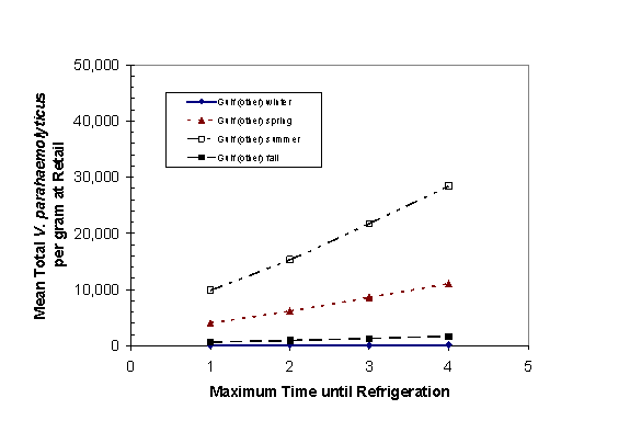
Figure A10-1. Predicted Effect of Maximum Time to Refrigeration with Conventional (Air-Circulated) Cooling of Oyster Shellstock (Gulf Coast, Non- Louisiana Harvest).

Figure A10-2. Predicted Effect of Maximum Time to Refrigeration with Conventional (Air-Circulated) Cooling of Oyster Shellstock (Gulf Coast, Louisiana Harvest).
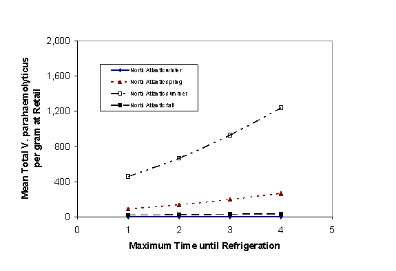
Figure A10-3. Predicted Effect of Maximum Time to Refrigeration with Conventional (Air-Circulated) Cooling of Oyster Shellstock (Northeast Atlantic Harvest).

Figure A10-4. Predicted Effect of Maximum Time to Refrigeration with Conventional (Air-Circulated) Cooling of Oyster Shellstock (Mid-Atlantic Harvest).
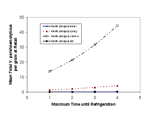
Figure A10-5. Predicted Effect of Maximum Time to Refrigeration with Conventional (Air-Circulated) Cooling of Oyster Shellstock (Pacific Northwest Dredged Harvest).
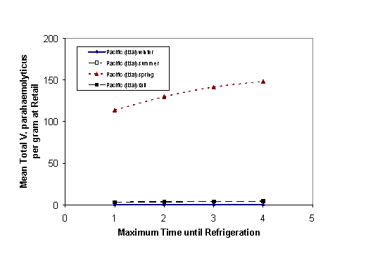
Figure A10-6. Predicted Effect of Maximum Time to Refrigeration with Conventional (Air-Circulated) Cooling of Oyster Shellstock (Pacific Northwest Intertidal Harvest).
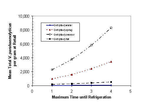
Figure A10-7. Predicted Effect of Maximum Time to Refrigeration with Rapid (on ice) Cooling of Oyster Shellstock (Gulf Coast, Non-Louisiana Harvest).
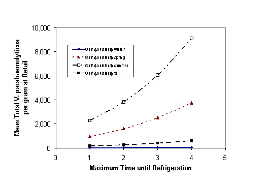
Figure A10-8. Predicted Effect of Maximum Time to Refrigeration with Rapid (on ice) Cooling of Oyster Shellstock (Gulf Coast, Louisiana Harvest).
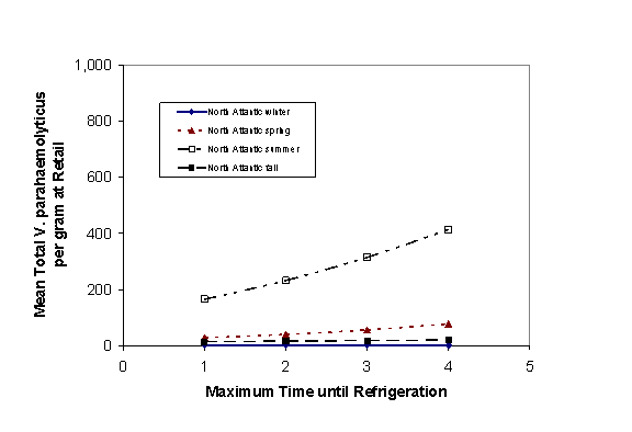
Figure A10-9. Predicted Effect of Maximum Time to Refrigeration with Rapid (on ice) Cooling of Oyster Shellstock (Northeast Atlantic Harvest).
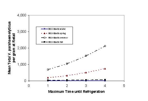
Figure A10-10. Predicted Effect of Maximum Time to Refrigeration with Rapid (on ice) Cooling of Oyster Shellstock (Mid-Atlantic Harvest).
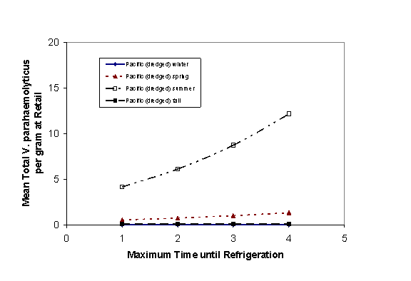
Figure A10-11. Predicted Effect of Maximum Time to Refrigeration with Rapid (on ice) Cooling of Oyster Shellstock (Pacific Northwest Dredged Harvest).
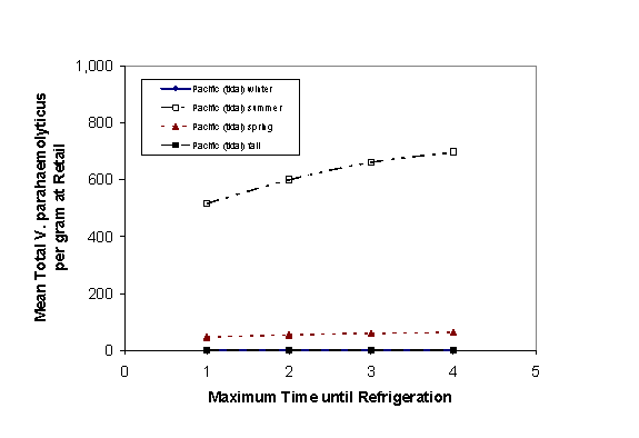
Figure A10-12. Predicted Effect of Maximum Time to Refrigeration with Rapid (on (on ice) Cooling of Oyster Shellstock (Pacific Northwest Intertidal Harvest).

Figure A10-13. Predicted Effect of Maximum Time-to-Refrigeration with Conventional (Air-Circulated) Cooling of Oyster Shellstock (Gulf Non- Coast, Louisiana Harvest).
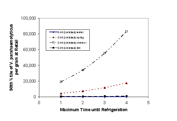
Figure A10-14. Predicted Effect of Maximum Time-to-Refrigeration with Conventional (Air-Circulated) Cooling of Oyster Shellstock (Gulf Coast Louisiana Harvest).
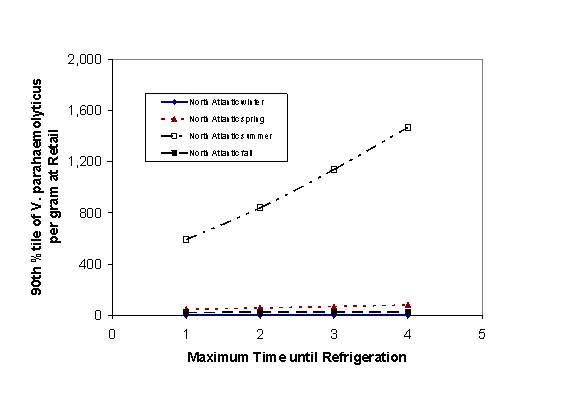
Figure A10-15. Predicted Effect of Maximum Time-to-Refrigeration with Conventional (Air-Circulated) Cooling of Oyster Shellstock (Northeast Atlantic Harvest).
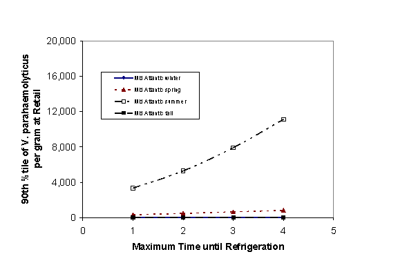
Figure A10-16. Predicted Effect of Maximum Time-to-Refrigeration with Conventional (Air-Circulated) Cooling of Oyster Shellstock (Mid-Atlantic Harvest).
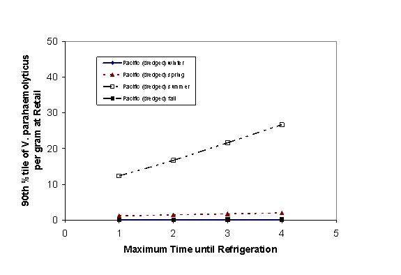
Figure A10-17. Predicted Effect of Maximum Time-to-Refrigeration with Conventional (Air-Circulated) Cooling of Oyster Shellstock (Pacific Northwest Dredged Harvest).
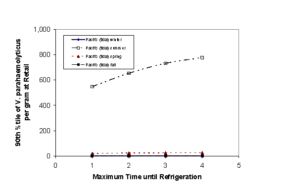
Figure A10-18. Predicted Effect of Maximum Time-to-Refrigeration with Rapid Conventional (Air Circulated) Cooling of Oyster Shellstock (Pacific Northwest Intertidal Harvest).
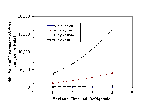
Figure A10-19. Predicted Effect of Maximum Time-to-Refrigeration with Rapid (on ice) Cooling of Oyster Shellstock (Gulf Coast, Non-Louisiana Harvest).
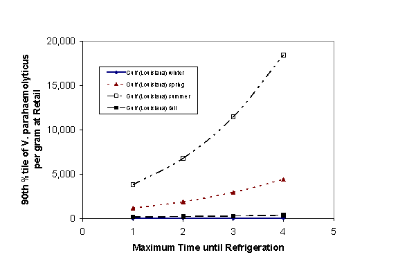
Figure A10-20. Predicted Effect of Maximum Time-to-Refrigeration with Rapid (on ice) Cooling of Oyster Shellstock (Gulf Coast, Louisiana Harvest).
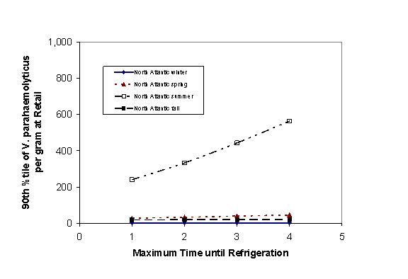
Figure A10-21. Predicted Effect of Maximum Time-to-Refrigeration with Rapid (on ice) Cooling of Oyster Shellstock (Northeast Atlantic Harvest).
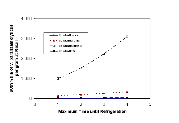
Figure A10-22. Predicted Effect of Maximum Time-to-Refrigeration with Rapid (on ice) Cooling of Oyster Shellstock (Mid-Atlantic Harvest).
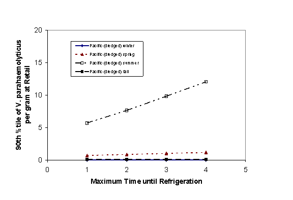
Figure A10-23. Predicted Effect of Maximum Time-to-Refrigeration with Rapid (on ice) Cooling of Oyster Shellstock (Pacific Northwest Dredged Harvest).
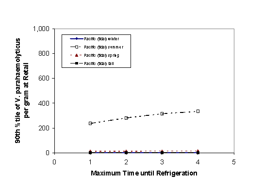
Figure A10-24. Predicted Effect of Maximum Time-to-Refrigeration with Rapid (on ice) Cooling of Oyster Shellstock (Pacific Northwest Intertidal Harvest).
Table A10-9 shows the impact of rapid cooling on ice on reducing the levels of V. parahaemolyticus with the corresponding decrease in risk per serving.
| Time-to-Refrigeration (h) | % reduction of total Vp/g | % reduction of risk per serving |
|---|---|---|
| 1 | 96.2% | 96.5% |
| 2 | 93.6% | 94.1% |
| 3 | 89.9% | 90.7% |
| 4 | 84.8% | 85.9% |
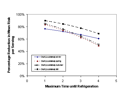
Figure A10-25. Predicted Effect of Maximum Time-to-Refrigeration with Conventional (Air-Circulated) Cooling of Oyster Shellstock (Gulf Coast, Louisiana Harvest).
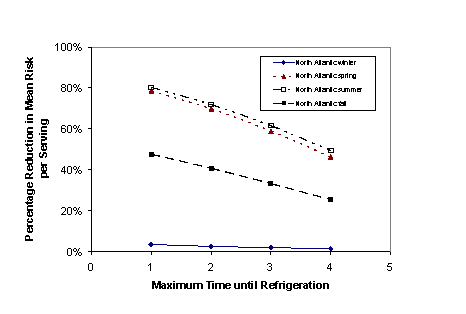
Figure A10-26. Predicted Effect of Maximum Time-to-Refrigeration with Conventional (Air-Circulated) Cooling of Oyster Shellstock (Northeast Atlantic Harvest).
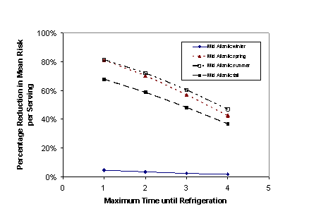
Figure A10-27. Predicted Effect of Maximum Time-to-Refrigeration with Conventional (Air-Circulated) Cooling of Oyster Shellstock (Mid-Atlantic Harvest).
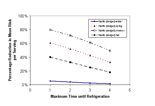
Figure A10-28. Predicted Effect of Maximum Time-to-Refrigeration with Conventional (Air-Circulated) Cooling of Oyster Shellstock (Pacific Northwest Dredged Harvest).
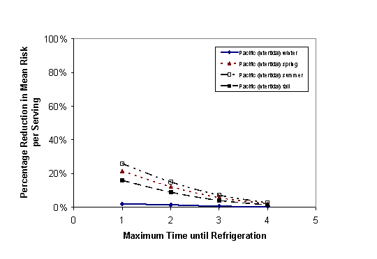
Figure A10-29. Predicted Effect of Maximum Time to Refrigeration with Conventional (Air-Circulated) Cooling of Oyster Shellstock (Pacific Northwest Intertidal Harvest).
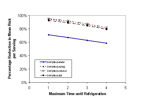
Figure A10-30. Predicted Effect of Maximum Time-to-Refrigeration with Rapid (on ice) Cooling of Oyster Shellstock (Gulf Coast, Non-Louisiana Harvest).
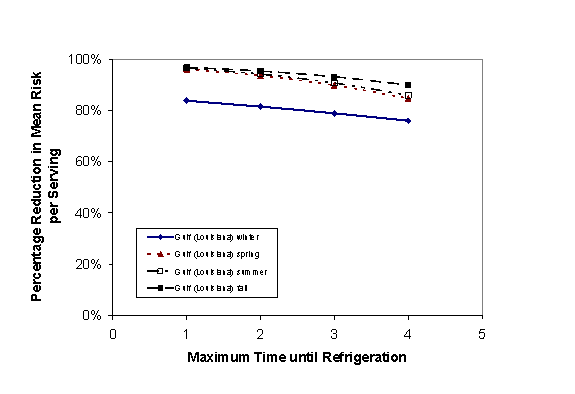
Figure A10-31. Predicted Effect of Maximum Time-to-Refrigeration with Rapid (on ice) Cooling of Oyster Shellstock (Gulf Coast, Louisiana Harvest).
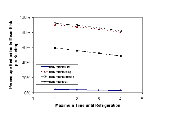
Figure A10-32. Predicted Effect of Maximum Time-to-Refrigeration with Rapid (on ice) Cooling of Oyster Shellstock (Northeast Atlantic Harvest.)
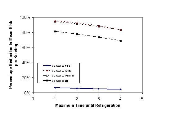
Figure A10-33. Predicted Effect of Maximum Time-to-Refrigeration with Rapid (on ice) Cooling of Oyster Shellstock (Mid-Atlantic Harvest.)
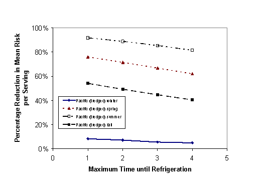
Figure A10-34. Predicted Effect of Maximum Time to Refrigeration with Rapid (on ice) Cooling of Oyster Shellstock (Pacific Northwest Dredged Harvest)
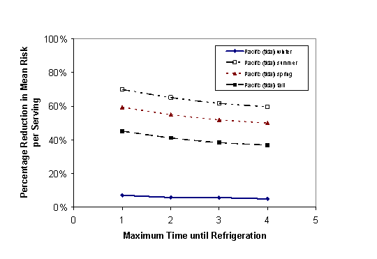
Figure A10-35. Predicted Effect of Maximum-Time-to Refrigeration with Rapid (on ice) Cooling of Oyster Shellstock (Pacific Northwest Intertidal Harvest).
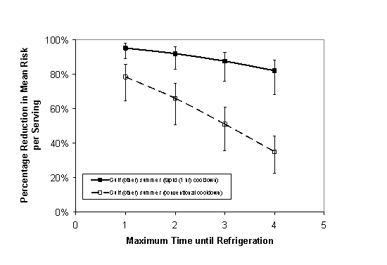
Figure A10-36. Rapid (on ice) Cooling versus Conventional (Air-Circulated) Cooling of Oyster Shellstock (Gulf Coast, Non-Louisiana Summer Harvest).

Figure A10-37. Rapid (on ice) Cooling versus Conventional (Air-Circulated) Cooling of Oyster Shellstock (Gulf Coast, Louisiana Summer Harvest).

Figure A10-38. Rapid (on ice) Cooling versus Conventional (Air-Circulated) Cooling of Oyster Shellstock (Northeast Atlantic Summer Harvest).
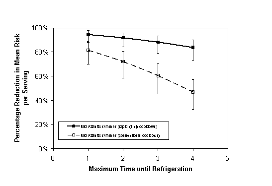
Figure A10-39. Rapid (on ice) Cooling versus Conventional (Air-Circulated) Cooling of Oyster Shellstock (Mid-Atlantic Summer Harvest).
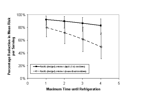
Figure A10-40. Rapid (on ice) Cooling versus Conventional (Air-Circulated) Cooling of Oyster Shellstock (Pacific Northwest Summer Dredged Harvest).
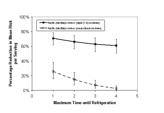
Figure A10-41. Rapid (on ice) Cooling versus Conventional (Air-Circulated) Cooling of Oyster Shellstock (Pacific Northwest Summer Intertidal Harvest).
The impact on illness and effect on harvest at different V. parahaemolyticus guidance levels for "at harvest" control was evaluated in Chapter VI of the technical document. It was recognized that deviation from compliance with these harvest guidance levels can occur in any region and season. The Louisiana Gulf Coast Summer harvest was selected as the region/season combination for illustrative example because the Gulf has the highest summer temperatures and Louisiana has the longest potential time for having oysters out of the water.
Selected levels of deviation from compliance (ranging from 0 to 50%) with different guidance levels (ranging from 100 to 100,000/g) were evaluated. The analyses were accomplished by altering the baseline model to represent the potential effect of the different levels of deviation from compliance. In other words, the impact of the different guidance levels determined in the above evaluation of the 10,000 V. parahaemolyticus/g was used as the 100% compliance (or 0% deviation from compliance) control and the outcome when 0, 10, 30, or 50% of the oysters containing more V. parahaemolyticus/g than the guidance level in question were allowed to reach the consumer. As seen in Table A10-10, the lower the standard level in question, the greater the impact of deviation from compliance on both percentage illnesses averted and loss of oyster harvest. At an "at-harvest" guidance level of 100 V. parahaemolyticus/g, a 30% deviation from compliance only reduces illness by 82% as compared to the 98% reduction predicted if 100% compliance were met.
At 10,000 and 100,000 V. parahaemolyticus/g the differences in illness reduction between 100% compliance and 70% compliance are not large. Therefore, as demonstrated in Figures A10-19 to A10-23, as the level of the microbiological criterion increases, the impact of compliance is less important. Conversely, strict microbiological criteria must be matched with a high level of compliance if they are to be effective.
| Total Vp/g At Time of Harvesta | Compliance Levelb | Reduction in Mean Risk per Serving (%) | Harvest Diverted (%)c | Illness Averted (%)d |
|---|---|---|---|---|
| 100/g | 50% | 47.7% | 33.0% | 64.9% |
| 70% | 66.7% | 46.2% | 82.1% | |
| 90% | 85.7% | 59.4% | 94.2% | |
| 100% | 95.3% | 66.0% | 98.4% | |
| 1000/g | 50% | 29.6% | 10.6% | 37.3% |
| 70% | 41.3% | 14.9% | 50.4% | |
| 90% | 53.0% | 19.1% | 62.6% | |
| 100% | 58.9% | 21.3% | 68.2% | |
| 5000/g | 50% | 11.4% | 2.8% | 14.4% |
| 70% | 15.9% | 3.9% | 19.9% | |
| 90% | 20.4% | 5.1% | 25.4% | |
| 100% | 22.7% | 5.6% | 28.1% | |
| 10,000/g | 50% | 6.4% | 1.4% | 8.2% |
| 70% | 8.9% | 2.0% | 11.4% | |
| 90% | 11.4% | 2.6% | 14.6% | |
| 100% | 12.7% | 2.9% | 16.2% | |
| 100,000/g | 50% | 0.57% | 0.12% | 0.79% |
| 70% | 0.77% | 0.17% | 1.11% | |
| 90% | 0.99% | 0.22% | 1.43% | |
| 100% | 1.10% | 0.25% | 1.58% |
a Assumes that the level of Vibrio parahaemolyticus
(Vp) is known in oysters at the time of harvest.
b The compliance level is the percentage oyster
harvest, which is removed from the raw oyster consumption market; this
percentage is assumed to have the same distribution of Vp/g as under the
baseline (no mitigation) scenario.
c Refers to the harvest that would need to be diverted
from the "raw market". d Assuming that the volume of product available for raw
consumption is impacted (i.e., reduced) according to the estimate of the % of
harvest lost from the raw market.
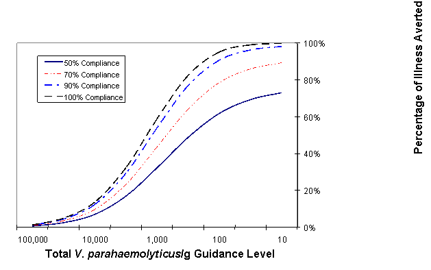
Figure A10-42. Percentage of Illnesses Averted
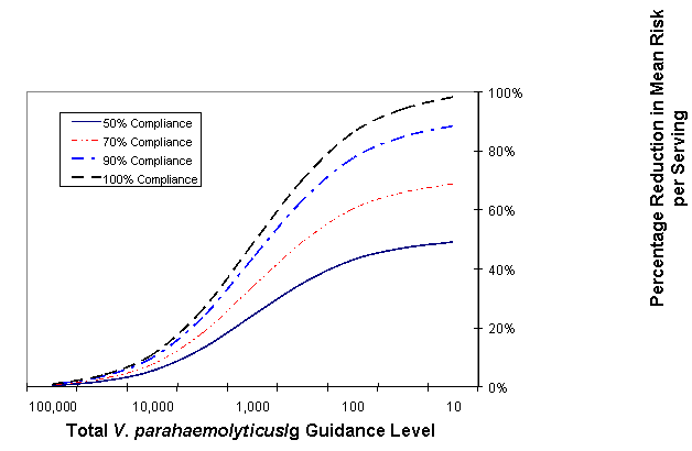
Figure A10-43. Percentage Reduction in Mean Risk per Serving
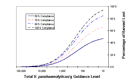
Figure A10-44. Percentage of Oyster Harvest Diverted from the "Raw Market" or Subjected to Preventive Controls.
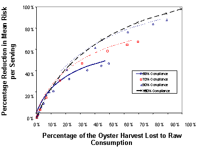
Figure A10-45. Percentage Reduction in Mean Risk per Serving versus Percentage of Harvest Diverted from the "Raw Market" or Subjected to Preventive Controls
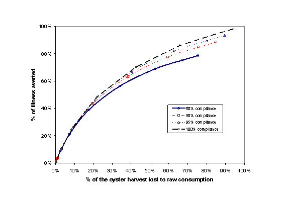
Figure A10-46. Percentage of Illnesses Averted versus Percentage of Harvest Diverted From the "Raw Market" or Subjected to Preventive Controls.
The impact of deviation from compliance at retail was evaluated in a similar manner to that at harvest. Selected levels of deviation from compliance (ranging from 0 to 50%) with different guidance levels (ranging from 100 to 100,000/g) was evaluated. Impact of deviation from compliance at retail is much higher at the higher standard levels at retail compared to that of at-harvest deviation from compliance (compare Tables A10-4 and A10-5). As seen in Table A10-5, like deviation from compliance at harvest, the lower the standard level in question, the greater the impact of deviation from compliance on loss of oyster harvest to the raw market. However, in the case of illness, deviation from compliance at retail appears to have a greater impact when the guidance level is high, even though a compliance rate of 100% does not result in 100% reduction in illness. At a retail guidance level of 100 V. parahaemolyticus/g, a 30% deviation from compliance reduces illness by approximately 90% as compared to the ~100% reduction predicted if 100% compliance were met. A rate of 50% deviation from compliance would result in approximately 74% reduction in illness versus the ~100% predicted if 100% compliance were met. If the guidance level was increased to 5, 000 V. parahaemolyticus/g, 50% compliance results in a larger decrease in the reduction of illness (approximately 63%) compared to ~100% predicted if there was 100% compliance.
At 10,000 and 100,000 V. parahaemolyticus/g the differences in illness reduction between 100% compliance and 70% compliance are larger than at 100 or 1,000. Therefore, as demonstrated in Figures A10-24 to A10-27, as the level of the microbiological criterion increases, the impact of compliance is more important on illness. Conversely, strict microbiological criteria must be matched with a high level of compliance if they are to be effective.
A deviation from compliance rate of 30% would substantially impact the reduction in risk of illness per serving (Table A10-11) for the higher guidance criteria. It is interesting to note that like at-harvest guidance, at 50% deviation from compliance of the lower guidance levels (100 and 1,000 V. parahaemolyticus/g), although the harvest is reduced by half of that at 100% compliance, reduction in illness is not equivalent. At the higher guidance levels, reduction in illness at 50% deviation from compliance is closer to half that at 100% compliance.
| Total Vp/g At-Retaila | Compliance Levelb | Reduction in Mean Risk per Serving (%) | Harvest Diverted (%)c | Illness Averted (%)d |
|---|---|---|---|---|
| 100/g | 50% | 50.0% | 49.0% | 74.5% |
| 70% | 70.1% | 68.6% | 90.6% | |
| 90% | 90.0% | 88.2% | 98.8% | |
| 100% | ~100% | 98.0% | ~100% | |
| 1000/g | 50% | 50.0% | 43.5% | 71.7% |
| 70% | 70.0% | 60.9% | 88.3% | |
| 90% | 90.0% | 78.3% | 97.8% | |
| 100% | ~100% | 87.0% | ~100% | |
| 5000/g | 50% | 49.8% | 34.5% | 67.1% |
| 70% | 69.9% | 48.3% | 84.4% | |
| 90% | 89.7% | 62.1% | 96.1% | |
| 100% | 99.6% | 69.0% | 99.9% | |
| 10,000/g | 50% | 49.5% | 29.7% | 64.6% |
| 70% | 69.4% | 41.5% | 82.1% | |
| 90% | 89.2% | 53.4% | 96.0% | |
| 100% | 99.0% | 59.3 | 99.7% | |
| 100,000/g | 50% | 45.3% | 13.9% | 53.4% |
| 70% | 63.4% | 19.4% | 71.2% | |
| 90% | 781.6% | 25.0% | 86.9% | |
| 100% | 90.6% | 27.8% | 94.1% |
a Assumes that the level of Vibrio parahaemolyticus
(Vp) is known in oysters at the time of harvest.
b The % of non-compliant oyster
harvest which is removed from the raw oyster consumption market; non-compliant
oyster harvest consumed raw is assumed to have the same distribution of Vp/g
as (above the compliance level) as under the baseline (no mitigation)
scenario.
c Refers to the harvest that would need to be diverted
from the "raw market".
d Assuming that the volume of product available for raw
consumption is impacted (i.e., reduced) according to the estimate of the % of
harvest lost.
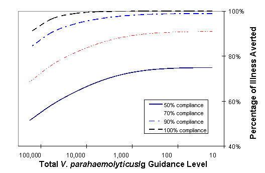
Figure A10-47. Percentage of Illnesses Averted
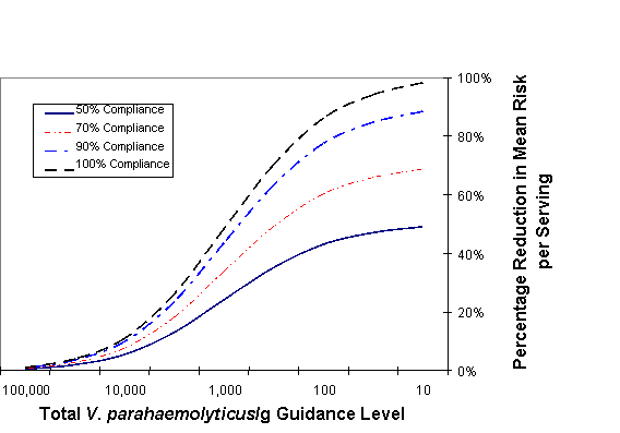
Figure A10-48. Percentage Reduction in Mean Risk per Serving.
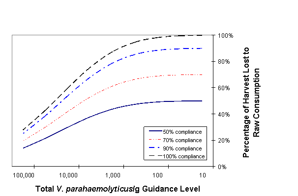
Figure A10-49. Percentage of Oyster Harvest Lost to Raw Consumption Market
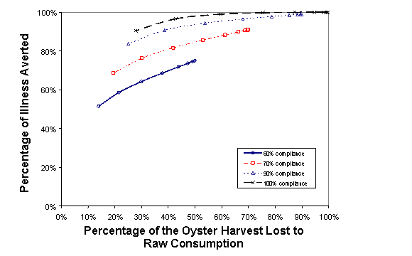
Figure A10-50. Percentage of Illnesses Averted versus Percentage of Harvest Lost to Raw Consumption Market
| Total Vp/g At-Retaila | Compliance Levelb | Reduction in Mean Risk per Serving (%) | Harvest Diverted (%)c | Illness Averted (%)d |
|---|---|---|---|---|
| 100/g | 50% | 50.0% | 47.0% | 73.5% |
| 70% | 70.0% | 65.8% | 89.7% | |
| 90% | 90.0% | 84.6% | 98.5% | |
| 100% | ~100% | 94.0% | ~100% | |
| 1000/g | 50% | 49.7% | 37.4% | 68.6% |
| 70% | 69.8% | 52.3% | 85.6% | |
| 90% | 89.9% | 67.2% | 96.7% | |
| 100% | 99.8% | 74.7% | ~100% | |
| 5000/g | 50% | 49.3% | 26.4% | 62.8% |
| 70% | 69.1% | 36.9% | 80.6% | |
| 90% | 88.8% | 47.5% | 94.2% | |
| 100% | 98.6% | 52.8% | 99.5% | |
| 10,000/g | 50% | 48.4% | 21.5% | 59.8% |
| 70% | 68.1% | 30.1% | 77.9% | |
| 90% | 87.5% | 38.7% | 92.6% | |
| 100% | 97.2% | 43.0% | 98.6% | |
| 100,000/g | 50% | 39.7% | 8.3% | 45.6% |
| 70% | 55.4% | 11.7% | 62.0% | |
| 90% | 71.4% | 15.0% | 77.2% | |
| 100% | 79.4% | 16.7% | 84.4% |
a Assumes that the level of Vibrio parahaemolyticus
(Vp) is known in oysters at the time of harvest.
b The compliance level is the percentage oyster
harvest, which is removed from the raw oyster consumption market or subjected
to preventive controls; this percentage is assumed to have the same
distribution of Vp/g as under the baseline (no mitigation) scenario.
c Refers to the harvest that would need to be diverted
from the "raw market" or subjected to preventive controls.
d Assuming that the volume of product available for raw
consumption is impacted (i.e., reduced) according to the estimate of the % of
harvest lost from the raw market or subjected to preventive controls.
In summary, as the levels increase, the percentage compliance for the at-harvest guidance is not as important in part because fewer numbers of illnesses are prevented at the higher guidance levels. When these same guidance levels are applied at-retail, however, a high percentage of illnesses is prevented, even when compliance is not 100%. For example, to obtain a 60% reduction in illness rates (assuming 50% compliance), the guidance level would need to be 100 at-harvest but at-retail could be as high as 10,000 V. parahaemolyticus/g.