Calibration of Intercity Trip Time Value with a Network Assignment Model: A Case Study for the Korean NW-SE Corridor

Iljoon Chang
Gang-Len Chang*
University of Maryland, College Park

ABSTRACT

This paper presents an innovative method for estimating the value of time (VOT) for intercity travelers with aggregate mode choice and origin-destination distribution data. The proposed method employs a network structure to capture the temporal and spatial interrelations of daily intercity trips among competing transportation modes. It is grounded on the assumption that the current trip and mode distributions in a regional corridor are close to a "user-optimum" state, where all tripmakers have nearly perfect information about the fares and schedules of all competing transportation modes and mostly employ the criterion of minimum total trip cost in their tripmaking decision. One can thus compare the current market share of each transportation mode with the estimated results to identify the best-fit VOT distribution. To realistically capture the competing environment for intercity trip decisions, the proposed method has incorporated not only the system performance factors (e.g., speed, capacity, and fare) in the modeling structure, but has also formulated the VOT as a distribution rather than a constant value across all system users. With the data from the northwest-southeast corridor of Korea, we have demonstrated that our proposed method has the potential to circumvent the need to estimate time value with disaggregate surveys.

INTRODUCTION

Despite the well-recognized role of value of time (VOT) in tripmaking decisions (e.g., departure time, route choice, and the selection of transportation modes), finding a reliable method for estimating VOT for a target population remains a challenging task. Over the past several decades, a large body of research has focused on this issue, mostly addressing it in terms of tripmaking behavior (Bruzelius 1979; Watson 1974; Moses and Williamson 1963; Hensher 1977; Earp et al. 1976) or from a microeconomic perspective (Jara-Diaz 1998; Gonzalez 1997; Gronau 1976; Senna 1994; Stopher 1976). For instance, one popular method for contending with this issue is to use stated preference and/or revealed preference from the disaggregate survey data. Such approaches, although theoretically appealing, are difficult to put in practice because of the high survey cost and potentially significant sampling as well as nonsampling survey errors. The quality of behavior-related surveys is difficult to control in developing countries due to low response rates and sample sizes that are insufficient for rigorous and unbiased analysis.

In contrast to the lack of data at a disaggregate level, aggregate data such as trip origin-destination (OD), fare, and travel time are mostly available from the operating agency of each transportation mode. For instance, we found in the study of high-speed rail (HSR) in Korea that market share information for each transportation mode for each OD is quite complete and reliable at the aggregate level. Thus, to circumvent the difficulties and costs associated with performing new disaggregate surveys, we developed a network-based method that can take full advantage of these valuable data for VOT estimation as well as HSR market share prediction. This paper will focus on our proposed network-based method for the calibration of VOT for tripmakers in the northwest-southeast (NW-SE) corridor of Korea.

BACKGROUND AND SYSTEM CHARACTERISTICS OF THE KOREAN TRANSPORTATION NETWORK

The NW-SE transportation network is in the most populous region of Korea, which is to be served by the new HSR system. As shown in figure 1, the NW-SE corridor connects major cities in Korea, including Seoul, Daejeon, Daegoo, and Busan. Between each city pair along this corridor, both the highway and the conventional rail networks are available. The airline system, however, is available only between Seoul, Daegoo, and Busan.

As shown in table 1, the total length of the NW-SE highway network along this corridor is 267.50 miles. Seoul and Daejeon are connected through a 95.25-mile-long highway. From Daejeon to Daegoo, a four-lane highway runs about 88 miles (table 2). The last segment, from Daegoo to Busan, is a four-lane highway of 83.94 miles. The NW-SE railway network is mostly parallel to the highway network and has about the same trip distance.

All the aggregate datasets for the calibration of time values are available including current market share, fare, trip distance, capacity, and travel speed. Each dataset is presented briefly below. For more convenient comparison, table 3 converts the trip segments into OD pair numbers, and figure 2 shows the current weekday market shares of the airline, highway, and conventional rail modes along the NW-SE corridor for three OD pairs from Seoul. Among those three OD pairs, we consider three distances: short distance, middle distance, and long distance. The shortest distance trip from Seoul in the network is OD pair 1. The long-distance trip is OD pair 3, and the mid-distance trip is OD pair 2. Some trips such as OD pairs 4 and 6 are shorter than OD pair 1, but those trips are not considered in this market share comparison for the moment. As can be seen in figure 2, about the same percentage of tripmakers use the highway and the conventional rail modes for OD pair 1. As the trip distance increases, travel by air becomes increasingly attractive to tripmakers. In contrast, for long-distance trips (i.e., OD 3), tripmakers rarely use the highway system, and about 78% of the total trips are by air.

The current fare for each transportation mode by OD pair is shown in table 4 and in figure 3, which show that the highway fare is about 31% of the fare of the airline system, and the fare for conventional rail is about 52% of that of the air mode for OD 3. Although transportation system operators may charge different fares according to travel times and ages of travelers, this research focuses on the nondiscounted regular fare of each mode.

Table 5 summarizes travel time and daily capacity of conventional rail and air by trip segment. The capacity of the highway mode is assumed to be 2,200 passenger cars per hour per lane, and if one assumes that the highway is in use 18 hours per day from 6 am until midnight then the capacity is 39,600 passenger cars per day per lane. We further assume, for convenient computation, that each car carries one passenger. The capacity of the airline system is based on its actual service schedules and the available types of aircraft.

BASIC ASSUMPTIONS OF THE MODEL

This paper presents an innovative method for estimating VOT distribution among the competing transportation mode users along the NW-SE corridor of Korea. We assumed several key factors in this new method:

• Every trip began at 6 am and finished by midnight.
• Those who could not finish their trips within a one-day period were stored in a dummy city for new trips on the following day.
• Time periods (or time intervals) were established for every two-hour period, and a one-day trip had a total of nine time periods.
• For the highway system, we assumed that all vehicles were passenger cars and one passenger was in each vehicle. Buses and other modes available along the highway system were excluded in this research but can be added in subsequent research.
• Highway mode users were only concerned about their toll costs and ignored expenditures for fuel, maintenance, and other costs in making their modal choices. This assumption may distort the estimation, but the main purpose of our research is to introduce a new method to investigate VOT distribution, not to investigate the actual VOT distribution among tripmakers in a proposed area.

Although the assumptions above may hinder the ability to accurately capture real modal choice decisions on the proposed network, the purpose of our research is rather to introduce a new method to estimate VOT distribution of tripmakers. Once the network-based model is established, however, it is very easy to add or drop networks, transportation modes, and other variables such as gas, tolls, insurance, and maintenance costs.

CALIBRATION OF VOT DISTRIBUTION FOR CURRENT MODE USERS

Because VOT is one of the key unknown factors that determine a tripmaker's modal choice decision, we developed a network-based method for VOT calibration based on the current distribution of trips among available transportation modes.

Our method is based on the assumption that all tripmakers intend to minimize their own travel costs, which consist of both fares and travel times. Thus, the current market distribution among available transportation modes for all OD demands can be viewed as a "user-optimum" state similar to that in a traffic assignment context. The method described below employs the "user-equilibrium" notion from traffic assignment but uses a time-space network to capture temporal and spatial interactions among different competing transportation modes and OD demands.

More specifically, our proposed model was developed to capture the following key features of a regional corridor offering several competing transportation modes for travelers making intercity trips:

• tradeoff between travel time and fare for each transportation mode and among all competing transportation modes;
• capacity and operational constraints of each transportation mode in the model formulation;
• generalized trip costs, such as speed, access time, and competition among the modes, based on the performance level of all transportation modes;
• temporal and spatial relationships of trips departing at different origins at different times of a day; and
• variation of the VOT across the population rather than viewing it as a constant.

A detailed discussion of the proposed method for VOT calibration in the Korean NW-SE corridor is presented below.

Steps in Calibrating VOT Distributions

Step 1: Select the initial VOT parameters for the target population.

Step 2: Construct a time-space operations model within each transportation mode and between competing transportation modes to estimate the current trip distribution.

Step 3: Design a set of experimental scenarios with a list of candidate VOT parameters.

Step 4: Estimate the user-optimum state of trip distribution among current transportation modes with the existing software (T-2) under each experimental scenario (see appendix).

Step 5: Compute the VOT parameters for current users, based on the discrepancies between the projected and actual market shares of all transportation modes over all OD pairs under all experimental scenarios.

Selection of Initial VOT Parameters

Although it is fully recognized that VOT theoretically should be a marginal wage rate (Gonzalez 1997), there is no standard tool for its estimation without a reliable representation of the total income and budget for the entire economy. As an initial step in determining the optimal mean VOT parameter, we assumed that it must lie within the 10th and the 90th percentile range of the resident income distribution of the Korean residents in the NW-SE corridor.

Data from the Korean Statistics Bureau indicated that the mean monthly income of the Korean population along the NW-SE corridor was $2,248 in 1999, equivalent to an average income of 20¢ per minute. The 10th percentile of resident income is $563 per month, about 5¢ per minute, and the 90th percentile of resident income is $5,295 per month, or about 46¢ per minute.

Construction of the Time-Space Operations Network

Based on the datasets illustrated earlier, this step develops a time-space operations network of all available transportation modes in the regional corridor. As shown in figure 4, three transportation modes (air, highway, and conventional rail) and three airports (nodes 5, 6, and 7) are available in the NW-SE corridor of Korea. Station nodes 5, 8, and 12 are located in the same city (Seoul), denoted as city node 1 in the figure.

By incorporating the time-varying demand and the capacity constraint for each transportation mode over each link, it is possible to convert figure 4 into a time-space network that represents the supply-demand relationships within each transportation mode and between competing modes. Note that the demand constraints are based on the collected trips for each OD pair and the link capacity constraints are based on the capacity of each available transportation mode during each time interval. The time-space network can be illustrated in a two-dimensional plane where the x-axis stands for the location and the y-axis for time. The core modeling concepts of the time-space operations network are summarized as follows:

• Nodes along the horizontal axis show different locations of stations or cities in the network, while the vertical axis shows the lapse of time. Thus, connections along the horizontal axis represent the movements between different locations within the same two-hour time period. Connections along the vertical axis illustrate the movements between different time periods at the same location. Connections in the diagonal direction represent movements between different locations and across different time periods.
• Access and main links are specified in the network. Access links are used to connect trips from origin cities to station cities, including waiting times, and main links are used for connecting trips between station nodes.
• Link cost is considered as the general cost (i.e., fare and travel time) of the transportation mode on a main link and is computed as the sum of the out-of-pocket cost and the travel time cost (see equation 2 later in this paper). Cost of the access links captures waiting time before departure.
• Link capacity reflects the physical capacity constraint of each transportation mode at different time intervals and locations during its operation.
• Origin nodes capture those trips originating from each city and terminating at a set of potential destination cities over a time horizon.
• Dummy nodes capture trips that cannot be finished within a one-day time period and serve as a supplemental set of origin nodes for tripmakers continuing their journeys the next day.

With these standard network formation concepts, we constructed the time-space operational relation between competing transportation modes. An example of the time-space operations network for the air mode for three time periods is presented in figure 5. Node 1P1 stands for city node 1 (in Seoul) at time period 1. Trips are generated from the city node (i.e., 1P1), and waiting times in the air mode are captured in the access link connecting city node 1P1 and station node 5P1. The main link from the station node in Seoul at time period 1 (5P1) to the station node in Daegoo at time period 1 (6P1) represents the trips from Seoul to Daegoo by air. Since this service is scheduled and takes less than two hours, all such trips can be finished within the same time period. Tripmakers arriving at station node 6 in time period 1 will finish their trips at city node 3 (3P1) in the same time period.

Note that for the airline network, its time-space interrelations are identical during all periods, because all trips using this mode can be finished within one two-hour time period. In this research, each time period covers two hours (as stated earlier), based on the available aggregation of the OD demand data. Certainly, one can further divide the time period into 30-minute segments, for instance, if OD demand data are available for such short intervals.

Most trips via conventional rail cannot be completed within one time period due to this mode's slower travel speed; thus, its time-space operations vary from one period to the next as shown in figure 6. Trips are generated from the city node in Seoul at time period 1 (1P1). Just as in the air case, waiting times are captured in the access link connecting 1P1 and 12P1, which is the conventional rail station node in Seoul at time period 1. Because travel time from Seoul to Daegoo (OD 2) by the rail mode takes 182 minutes (as shown in table 5), the traveler will end up in Daegoo at time period 2 (14P2). Trips from Seoul to Busan take more than four hours, so trips starting from Seoul in time period 1 will arrive at Busan in time period 3 (15P3). One can follow the same procedures to construct the time-space operations network for the highway system as shown in figure 7.

All three sub-networks are then connected through their common demand nodes, as illustrated in figure 8, and constitute the entire operational network for the three transportation modes. For convenience, figure 8 only shows the demand from time period 1 and location node 1. Combining those three sub-networks reflects the fact that travelers in each OD pair can choose any of the three available transportation modes. In brief, the time-space network model is constructed with the following data:

• network topology;
• fare for each transportation mode;
• current trip demand between every OD pair;
• capacity of each transportation mode; and
• VOT probability density function (PDF) of the current travelers.

Note that a normal PDF starts with its parameters set to initial values, and these values are evaluated and redefined through the calibrating process. Also note that the demand node of figure 8 is an artificial node that simply generates demands.

As mentioned previously, with our time-space network relationship, current intercity trip distribution among transportation modes can be viewed as similar to the user-optimum state in the context of urban traffic assignment. Hence, similar algorithms for a user-optimal solution can be employed to solve the large time-space network and compute all estimated market shares between all OD pairs and transportation modes. The objective function of the proposed operational network is specified as follows:

It can further be expressed mathematically as

where x = x ( );

= out-of-pocket cost (or fare) from origin r to destination s using the path between i and j ;

= VOT;

= travel time from origin r to destination s using the path between i and j ; and

= total number of trips from origin r to destination s using the path between i and j .

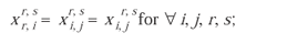
Note that each path in the time-space network actually represents the transportation mode selected by tripmakers, the passage of time from one time period to another, and the change in physical position from their origin point to their destination.

The constraints of the objective function are as follows:

1) Non-negative flow conditions:

2) [Trips on Link] ≤ [Total Outflow]:

3) [Total Trips]
= [Trips over Each Link on the Designated Link Path]

4) Link Usage Condition:

5) Continuity Conditions:

To ensure that the proposed model can realistically capture intercity mode choice behavior, we further tested the performance of our proposed model against three hypotheses.

Hypotheses for Performance Tests

Based on the collected dataset for the NW-SE corridor, it is expected that:

1. When mean VOT of the system users is high, most tripmakers will take the faster but more expensive transportation modes (e.g., air), especially for long-distance trips.
2. When mean VOT of the system users is low, most tripmakers will take the slowest but least expensive transportation mode (i.e., highway).
3. Mean VOT of tripmakers who prefer to take the conventional rail system is expected to lie between that of the air and the highway system users, because the direct cost and travel speed of the conventional rail system is between those of air and highway.

The following experimental scenarios were used to evaluate whether the proposed model's performance was consistent with those hypotheses. To test the hypotheses, we used the initial VOT distribution and a standard deviation of 0.02, which is currently the standard deviation of resident income distribution in the target area.

Case 1: Mean VOT of the system users is 5¢/min (the 10th percentile of the average resident income in the proposed area) with a standard deviation of 0.02.

Case 2: Mean VOT of the system users is 10¢/min with a standard deviation of 0.02.

Case 3: Mean VOT of the system users is 20¢/min (the average resident income in the proposed area) with a standard deviation of 0.02.

Case 4: Mean VOT of the system users is 25¢/min with a standard deviation of 0.02.

Case 5: Mean VOT of the system users is 35¢/min with a standard deviation of 0.02.

Case 6: Mean VOT of the system users is 40¢/min with a standard deviation of 0.02.

Case 7: Mean VOT of the system users is 46¢/min (the 90th percentile of the average resident income in the proposed area) with a standard deviation of 0.02.

Note that VOT in all cases was assumed to be normally distributed with a standard deviation of 0.02, based on the wage distribution in the target service area.

Test Results

Using our proposed network model in the aforementioned scenarios, the results, as expected, indicated that most tripmakers travel by air when their VOT is assumed to be high (Cases 5, 6, and 7) for long-distance (OD 3) trips. On the other hand, tripmakers use the highway mode when their VOT is assumed to be relatively low (Cases 1 and 2). This is consistent with our first hypothesis, and a graphical illustration of such relationships is presented in figures 9 and 10. In the case of conventional rail, figure 11 shows that some tripmakers are using this mode for long-distance trips (OD 3) when their VOT is assumed to be between 10¢/min (Case 2) and 20¢/min (Case 3). In contrast, travelers on short-distance trips prefer to take this mode when their VOT is assumed to be between 20¢/min (Case 3) and 25¢/min (Case 4). The results are also consistent with the second hypothesis; that is, low-income travelers tend to select slow and inexpensive transportation modes.

ESTIMATION OF OPTIMAL PARAMETERS FOR VOT DISTRIBUTION

Note that with the same assumptions for trip choice behavior and with identical system performance data (i.e., fare, travel speed, travel time, trip distance, and capacity), the scenario that yields the best fit for the current demand distribution must best capture the actual VOT distribution among tripmakers. Thus, by employing the network-based method presented in the previous section, we performed the preliminary search of the optimal parameters for the VOT distribution with those well-selected experimental cases.

Selection Criterion

To identify the best-fit VOT, we employed the weighted-average error of estimation as the criterion to compute the discrepancy between the estimated market and the current market shares. The computed value allowed us to select the set of mean VOT that best captured the current trip distribution among all available transportation modes. It is defined as follows:

• weighted-average error for mode m on OD pair i in scenario
   

where i = OD pair i;

m = transportation mode;

_{i, m} = actual volume of transportation mode m on OD pair i;

V_{i, m} = estimated volume of mode m on OD pair i in scenario; and

ABS = absolute value.

As such, the total weighted-average error in the scenario can be expressed as
 

where = total actual volume of the entire system, denoted as

Experimental Results

As shown in figure 12, among all candidate parameters Case 4 (mean VOT equal to 25¢/min) yielded the lowest weighted-average error of estimation. To further identify the best-fit mean VOT, we divided the range between Cases 3 (mean VOT = 20¢/min) and 4 (mean VOT = 25¢/min) into the following four additional cases:

Case 3-1: VOT is normally distributed with a mean of 21¢/min and a standard deviation of 0.02.

Case 3-2: VOT is normally distributed with a mean of 22¢/min and a standard deviation of 0.02.

Case 3-3: VOT is normally distributed with a mean of 23¢/min and a standard deviation of 0.02.

Case 3-4: VOT is normally distributed with a mean of 24¢/min and a standard deviation of 0.02.

With the same estimation procedures, we found that Case 3-4 (mean VOT 24¢/min) yielded the lowest estimation error, as presented in figure 13. Thus, for the purpose of market share prediction, it seems that a mean VOT of 24¢/min can reasonably represent the travel time value of transportation system users in the NW-SE corridor of Korea.

Estimation of the Best-Fit Standard Deviation

Given the best-fit mean VOT of 24¢/min, this section focuses on identifying the best-fit standard deviation for system users along the NW-SE corridor with five carefully identified cases: Cases A, B, C, D, and E summarized in table 6. The collected dataset shows that the standard deviation of the residential income of the proposed area is 0.02. Thus, we chose 0.02 as an initial standard deviation, and the upper bound becomes 0.25. As shown in table 6, Case A is the base case, with a standard deviation of 0.02, which is identical to Case 3-4 in figure 13. The estimation results of all five cases are illustrated in figure 14. It is apparent that Case C (standard deviation = 0.10), compared with the initial and other cases, yields the lowest weighted-average error of estimation for all system users.

In light of the above exploration, we conclude that tripmakers' VOT along the NW-SE corridor of the Korean transportation network is best approximated by a distribution with a mean of 24¢/min (Case 3-4, figure 13) and standard deviation of 0.10 (Case C, table 6). The estimated trip distributions of all transportation modes and OD pairs with the best-fit VOT parameters along with their weighted-average errors are presented in table 7.

Note that with the estimated VOT distribution, one can now reconstruct the entire corridor network with HSR and employ the same solution procedures to estimate the market share of HSR as well as other existing transportation modes. The same network relationship can also be employed to explore the impact of various operating policies, such as fare structure, on the potential market share of all competing transportation modes.¹

CONCLUDING COMMENTS

This paper presents a network-based method for estimating the VOT distribution for intercity transportation users. The proposed method is unique in its capability to take full advantage of available aggregate market share data and in its flexibility to incorporate all system performance factors as well as the competing nature of available transportation modes in the modeling structure. With such a method, it is possible to circumvent the need to perform costly disaggregate surveys at an individual level. It is often quite difficult to maintain quality control in such surveys, especially over the inevitable nonsampling errors that result from a variety of social and behavioral factors in developing countries. We expect that the proposed method will enable researchers to explore the complex interactions between all competing and/or new transportation modes from either a demand or system performance perspective with relatively reliable and available aggregate data.

REFERENCES

Bruzelius, N. 1979. The Value of Travel Time: Theory and Measurement. London, England: Croom Helm.

Chang, I.J. 2000. Optimizing Time-Varying Multiple Origin-Destination Trips Among Competing Modes in a Regional Corridor. Ph.D. dissertation. University of Maryland.

Earp, J.H., R.D. Hall, and M. McDonald. 1976. Model Choice Behaviour and the Value of Travel Time: Recent Empirical Evidence. Model Choice and the Value of Travel Time. Edited by I.G. Heggie. Oxford, England: Clarendon.

Gonzalez, R.M. 1997. The Value of Time: Theoretical Review. Transportation Reviews 17(3):245–266.

Gronau, R. 1976. Economic Approach to Value of Time and Transportation Choice. Transportation Research Record 587:1–11.

Hensher, D.A. 1977. Value of Business Travel Time. New York, NY: Pergamon.

Jara-Diaz, S.R. 1998. Time and Income in Travel Choice: Towards a Microeconomic Activity-Based Theoretical Framework. Theoretical Foundations of Travel Choice Modeling. New York, NY: Elsevier.

Moses, L.M. and H.F. Williamson, Jr. 1963. Value of Time, Choice of Mode, and the Subsidy Issue in Urban Transportation. Journal of Political Economy 71:247–264.

Senna, L.A.D.S. 1994. The Influence of Travel Time Variability on the Value of Time. Transportation 21:203–228.

Stopher, P.R. 1976. Derivation of Values of Time from Travel Demand Models. Transportation Research Record 587:12–18.

Watson, P.L. 1974. The Value of Time: Behavioral Models of Modal Choice. Lexington, MA: Lexington Books.

APPENDIX

T-2 Traffic Assignment Model

The T-2 traffic assignment model consists of the following principal components:

1. minimum path assignment,
2. probability of taking the mode,
3. bicriterion equilibrium assignment, and
4. T-2 algorithm.

1. Minimum-Path Assignment. The primary function of the model is to assign trips with a stochastic VOT on a network for fixed link times and costs.

Given:

trip matrix

network topology,

let

R ₊ = {positive real numbers}

N = {nodes in the network}

E = {links in the network}

Ground set:

A = ,

( ) = number of trips going from origin node O to destination node D with a VOT , and

( ) = flow on link e of trips that originated at origin node O with VOT .

Then, total flow on link of trips that originated from every possible origin with VOT is

Now, the feasible traffic assignment for a given trip matrix is

Also, equation (1) is rewritten as

where is the PDF of VOT for trips going from origin node O to destination node D.

2. Probability of Taking the Mode. The main purpose of the module is to compute the probability of taking one mode over all available transportation modes in a network corridor. The first step is to determine the range of the VOT parameter based on all feasible paths and then to determine the probability of taking each transportation mode, as follows:

where

L = lower limit of VOT

U = upper limit of VOT and

= PDF of VOT of trips from origin to destination.

3. Bicriterion Equilibrium Assignment. For a given topology, VOT, PDF, and OD matrices, the objective function is to minimize the total generalized cost function.

Objective:

The decision variable of the objective function is the total number of trips using link e that originate at node O, and is written as follows:

x_e = trips using link e that originate at origin node O

One needs the list of constraints to solve the objective function, and those constraints are summarized below.

Constraints:

The first constraint ensures the feasibility of the assignment. The second constraint is to ensure that the total trips on link e is the sum of all trips originating from different origins on the network but that use the same link. The third, fifth, and seventh constraints hold the positive trip numbers and travel times. The total number of trips on link e is the integral of all trips under different VOT scenarios. Lastly, constraint six shows that the travel time on link e is the sum of travel times on the link from different origins.

4. T-2 Algorithm. The T-2 algorithm used to determine the optimum mode choice and trip distribution is presented below.

Step A. Initialization

Do a T-2 minimum-path assignment to obtain

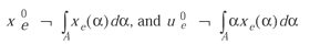
Step B. Ascent direction

Fix all link costs and times

and perform a T-2 min-path assignment to obtain

Step C. Termination test

Let

If

Quit

implies the e-approximate T-2 equilibrium traffic assignment.

Otherwise, go to Step D.

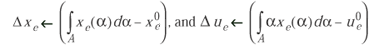
Step D. Determining step size

Let

If

Step E. Improved solution

Update all and ;

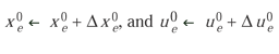
and return to Step B.

Address for Correspondence and End Notes

Gang-Len Chang, Department of Civil Engineering, University of Maryland, College Park, MD 20742. Email: gang@glue.umd.edu.

^1. For a detailed presentation of this topic, see Chang (2000).