(Appendices 1-4 available in PDF)
The FDA/FSIS Listeria monocytogenes risk assessment organizes currently available information on listeriosis. It was designed to examine broad groups of foods most likely to cause listeriosis; it does not determine whether a food category is 'safe.' We did not model the source or process of contamination of the food, but did include expected growth between retail and consumption. For frankfurters that are usually heated before consumption, the reheating step was modeled, to allow for those occasions where the food is not adequately heated to kill all microorganisms. The model provided a baseline or description of our best prediction of the role the selected foods play in the threat from listeriosis in the United States. The model did not attempt to evaluate any mitigations that might be imposed during the manufacturing of any specific foods to reduce the risk from listeriosis; this could be the objective of a subsequent risk assessment. However, this risk assessment model was used to estimate the likely impact of intervention strategies by changing one or more input parameters and measuring the change in the model outputs. These changes to the model, which are commonly referred to as 'what if' scenarios, can be used to test the likely impact of new or different processing parameters or regulatory actions. These 'what if' scenarios can also be hypothetical, not necessarily reflecting achievable changes but designed instead to show how different components of the complex model interact.
Another objective of this risk assessment was to collect information on the dose-response relationship and develop a model to estimate the likelihood of listeriosis from consuming specific numbers of L. monocytogenes.
This risk assessment provides an estimate of the degree of certainty associated with the data. To accomplish this, we used distributions of the data so that real differences that exist for an individual parameter would be represented instead of using point estimates or means. Contamination levels in different samples, amount consumed per servings, L. monocytogenes growth rates for foods within a group and lengths of storage time by the consumer are data that were considered in the model as distributions.
The risk assessment presents the scientific information, both what is known and the degree of certainty. Although the risk assessment uses the best data available, one of the important roles of the risk assessment is to determine critical absences of adequate data that drive the uncertainty in the overall risk assessment. Thus, risk assessment can be used as a link between risk management and research. Risk managers should consider uncertainty when evaluating the significance of a parameter. In some instances, uncertainty may be too large to allow making inferences from the risk assessment. The risk assessment does not impose a judgement or make value decisions based upon the information, that is the role for risk management.
The overall structure of the exposure assessment and dose-response models are depicted in figures A3-1 and A3-2, respectively.
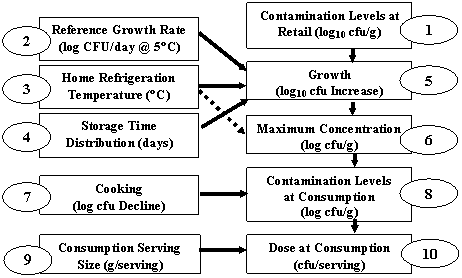
Figure A3-1. Flow chart of Listeria monocytogenes risk assessment model for individual exposure components. This part of the model was integrated with a two-dimensional simulation where one dimension characterized the variability among meals, while the second dimension characterized the uncertainty in the prediction. A different simulation was performed for each of the 23 food categories.
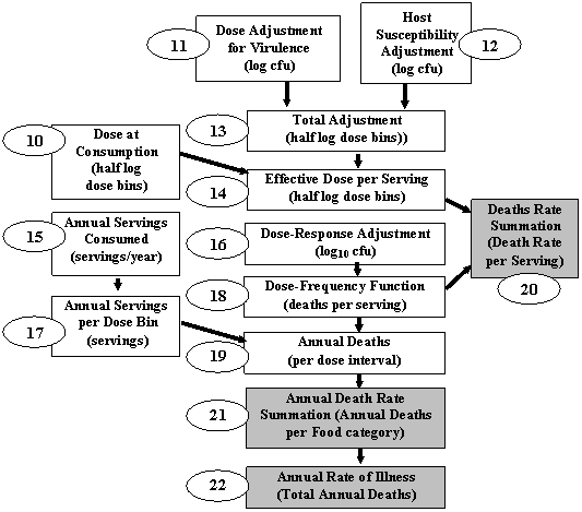
Figure A3-2. Flowchart of Listeria monocytogenes risk assessment calculation of population estimates. This part of the model was integrated with a one-dimensional Monte-Carlo, where the single dimension represents uncertainty. The subpopulations were modeled separately. The outputs of the model that appear in the hazard characterization steps are in dark gray boxes.
Figures A3-1 and A3-2 show the flow of the calculations used in the risk assessment.
Step 1. Distributions for contamination at retail for each food category.
Step 2. Distributions for the reference growth rate at 5°C for each food category.
Step 3. A distribution of home refrigerator temperatures in the United States- the same distribution was used for all food categories.
Step 4. Distributions for post-retail storage time for each food category.
Step 5. A growth model used for all food categories but was triggered only for servings with one or more bacterium. In this module, the exponential growth rate for the refrigeration temperature was calculated and multiplied by the storage time. The parameters included in the growth model were specific to the characteristics of the foods in each food category.
Step 6. The maximum concentration for each food category. Post growth L. monocytogenes concentrations were truncated at this level. The maximum growth was temperature dependent with more growth allowed at higher refrigeration temperatures.
Step 7. A model representing the effect of reheating frankfurters on L. monocytogenes concentration, used for frankfurters only.
Step 8. Net contamination at time of consumption. Calculated with inputs from steps 1, 6, and 7.
Step 9. Distributions of serving size for each food category.
Step 10. Distributions of dose at consumption for each food category. This is the final output of the 2D simulation. After collapsing the variability dimension to half-log dose bins, the output for each food category was conveyed to the 1D dose-response simulation for each population group.
Step 11. A distribution for variability of L. monocytogenes strain virulences in mice, with the implicit assumption that a similar range will be observed in humans.
Step 12. A distribution adjusting for variability in host susceptibility among humans, with three (High, Medium, Low) separate adjustments applied to represent different possible ranges. The adjustment increased the range of effective doses.
Step 13. The sum of the strain variability (step 11) and host susceptibility distributions (step 12) obtained by 2D Monte-Carlo, with 100,000 variability iterations and 300 uncertainty iterations. The variability dimension was then collapsed to half log dose bins.
Step 14. Summation of the exposure assessment (step 10) and adjustment factor (step 13) for each food category
Step 15. The annual number of meals consumed for each food category.
Step 16. Addition of the dose-response adjustment factor that is applied to make the predictions consistent with CDC estimates of the annual death rate attributable to the population group. For baseline calculations this value was recalculated for every uncertainty iteration. For subsequent evaluations (i.e. intervention analysis) the values established for each iteration for the baseline were retained.
Step 17. An intermediate calculation of the number of annual servings falling in each dose bin for each food category. This was obtained by multiplying the number of servings (step 15) by the fraction falling in each effective dose bin (step 14).
Step 18. Calculation of the death rate per serving for each dose bin (from step 14), using the dose-response function derived from mouse data.
Step 19. An intermediate calculation of the number of annual deaths for each dose bin and food category. This was obtained by multiplying the death rate per serving (step 18) by the number of servings for the dose bin (step 17).
Step 20. Calculation of the death rate per serving for each food category by summing across dose bins. This was obtained by summing the product of the death rate (step 18) and serving fraction (step 14) across all bins.
Step 21. Calculation of the annual number of deaths for each food category by summing across dose bins (step 19).
Step 22. Calculation of the total number of deaths by summing across food categories.
A risk assessment framework separates the assessment activities into four components; hazard identification, exposure assessment, dose-response assessment (hazard characterization), and risk characterization. This framework allows organization of a highly complex array of varied data, characterization of the predicted consequences, definition of uncertainties, and identification of data gaps.
Hazard Identification is one interface between risk assessment and risk management where the problems that the assessment is intended to address are identified and specific questions about model design are resolved. Endpoints in this assessment include death and serious illness for the intermediate-age subpopulation and two readily identifiable vulnerable subpopulations: perinates (fetuses and newborns) and the elderly (60 years of age and older).
Exposure related to foodborne L. monocytogenes consumption can be separated into two main subcategories: pathways of contamination and frequency of consumption of contaminated foods. This risk assessment did not consider the pathway of contamination or any events occurring prior to retail. The exposure assessment emphasized modeling foods that have a potential for L. monocytogenes contamination at retail. The development of the exposure assessment included:
Identification of ready-to-eat foods that are known to have been associated with L. monocytogenes from outbreaks, sporadic cases, and national and international recalls and other sources. Foods with a history of L. monocytogenes concentration were also evaluated.
Food categories, grouped according to primary origin, epidemiological and surveillance experience, processing operations and food characteristics, and the availability of consumption and contamination data or useable proxy data.
Development of distributions of the amount consumed per serving for each food category and estimates of the annual number of servings in U.S. using national food consumption surveys and other food consumption and census information.
Calculation of distributions of contamination levels at retail for each food category, based on published studies of naturally-occurring L. monocytogenes contamination. For contamination data of foods after manufacture, growth to the retail store was estimated.
Modeling of data to describe the opportunity for growth, decline, or inactivation of L. monocytogenes between the time that a food was purchased and the time it was consumed.
Development of a mathematical model to represent reheating of frankfurters in the home. Normally a cooking or reheating step will kill vegetative microorganisms.
Derivation of distributions of contamination levels at consumption for each food category, based on initial L. monocytogenes contamination, growth potential, storage duration, refrigeration temperatures and reheating.
Derivation of estimates of the frequencies and levels of contamination of a serving, by combining distributions of food consumption frequency and amount with distributions of food contamination frequency and levels.
Because of a lack of data, foods prepared outside the home were not modeled separately. The food consumption survey data included all eating occasions within and outside the home. It was therefore assumed that contamination at retail, refrigeration temperature, and storage times included the meals served or prepared outside of the home (restaurant and food service meals).
For L. monocytogenes, the overall incidence of severe illness, and predicted relative risk to age-related susceptible subpopulations are well characterized. The relation between the amount of L. monocytogenes consumed (dose) and the likelihood or severity of resultant illness from that dose (response) is not well understood. The dose-response effect is a complex function of the number of pathogens consumed, their level of expressed virulence, the food matrix that the pathogen is in, and the susceptibility and immunity of the human host.
For this L. monocytogenes risk assessment the following information was considered:
Accumulating epidemiological information indicates that different strains of L. monocytogenes vary in their ability to cause illness. Data were utilized from animal studies that compare the virulence of L. monocytogenes strains isolated from humans and from foods in order to describe the distribution of virulence among strains encountered in foods.
Immunological and physiological factors in humans determine the distribution of susceptibility that may be found throughout a population.
Food matrix effects have been theorized to affect the ability of a pathogen to survive inside the body (e.g., the fat content of foods appears to affect the infectious dose of Salmonella sp.). Quantitative data specifically related to L. monocytogenes in humans were not available.
Epidemiological data with the number of deaths in each population per year and the ratio of serious illness/deaths.
The probability of illness in three different subpopulations of consumers is described; perinatal (with exposure occurring in utero from foodborne infection of the mother during pregnancy); elderly (60 years of age and older); and intermediate-age subpopulation, which includes both healthy and immunocompromised individuals (but excludes the other two subpopulations). A host susceptibility adjustment was applied to each of the three subpopulation curves. The adjustments used animal data to establish a susceptibility range and human epidemiological surveillance data to adjust for increased susceptibility of these subpopulations.
Risk characterization integrates the distributions generated in the exposure assessment and the hazard characterization. The published literature provides an estimate of the number of illnesses and deaths attributed to L. monocytogenes. Therefore, the primary component of this risk characterization is a probabilistic estimate of the likelihood of illness from consumption of contaminated food from each of the 23 food categories.
The risk characterization section of this risk assessment provides the results of the assessment, and the associated uncertainty around those results. Additionally, data gaps, which, if filled, would contribute to reducing the uncertainty in the assessment, are identified to highlight critical needs for additional research.
Monte-Carlo simulations are an integral part of most quantitative risk assessments. They include repetitive calculations with minor variations and are made possible by the development of the computer.
The exposure assessment portion (see Figure A3-1) of this risk assessment model employs a two-dimensional Monte-Carlo simulation. One dimension represents variations associated with the capacity of individual servings of food to cause listeriosis. Sources of variation modeled include L. monocytogenes concentration at the retail level, amount consumed per serving, microbial growth rates, product storage times and temperatures, strain virulence, and host susceptibility. The second dimension represents the uncertainty in the predictions made. This is described more fully below.
The dose-response portion (see Figure A3-2) of the risk assessment employ a one-dimensional Monte-Carlo simulation, where the range of predicted values represent uncertainty only. In this part of the assessment, the U.S. population is modeled as a whole, beginning with the estimate of the fraction of servings falling in particular dose ranges from the first part of the risk assessment.
The results of the FDA/FSIS L. monocytogenes risk assessment are based on statistical calculations. Thus the parameters modeled by this risk assessment are represented by distributions of values. These distributions represent either the known variation or uncertainty about a quantitative value. As a result, instead of using deterministic calculations (adding or multiplying single values, usually means), this risk assessment uses simulation modeling techniques, i.e., Monte Carlo modeling, to make its calculations. In this technique, the model is repeatedly calculated and in each iteration the process picks a new value from each of the distributions. This means that there is not a single answer to the calculation; instead, a distribution of calculated values is generated.
Mathematical calculations with distributions do not always form simple symmetrical normal distributions. Many distributions are asymmetrically skewed with long tails on one side. When any two independent distributions are added the resulting distribution has a larger variance than either original distribution, and may not be of the same shape as either of the original distributions. When distributions are multiplied, skewed distributions often result with a tail extending toward larger values. The magnitude of the variance for the product of two distributions is typically larger than the variances of the original distributions. The practical effect of this is that multi-step calculations have increasingly wider output distributions. This occurs whether the distribution describes variation or uncertainty.
A skewed distribution does not have the same value for the mean and the median (half of the values above and half are below that value) as does the normal distribution. In extremely skewed distributions, the median is frequently considered a better parameter than the mean to represent the distribution, because it is not as affected by extreme values as the mean. However, summing the median values for two or more distributions does not equal the median of the summed distributions.
Variability
Variability is real variation in the individual members of a population or system with which a decision-maker is concerned. It cannot be eliminated by improved measurement technique. It is information the decision-maker needs. A distribution describing variability describes the frequency of occurrence.
When statistical distributions are used, the distinction between variability and uncertainty is in some circumstances contextual, and depends on the question which is being answered. Variability which is present in the experiment that is not also present in the real world circumstances with which the decision-maker is concerned is a source of uncertainty. Uncertainty reflects imperfections in our knowledge about what is real. It can be reduced through additional research. Although, the decision-maker should want to know the extent of the uncertainty associated with a calculation, he/she would prefer not to have it. A distribution describing uncertainty describes the likelihood or expectation of occurrence. There is often very little basis for segregating true variability from experimental error, where the former is expected to be reproduced in the problem at hand, while the latter is not. The extent of the variability is quite often itself a source of uncertainty.
Adaptation of a Monte-Carlo simulation process to provide for separate accounting of both variability and uncertainty requires modification of both the front and back ends of the procedure. The descriptive statistics used to describe the variance for each of the data sets must have separate distributions for each source. The output from the iteration collection procedure must have two dimensions: one for variability, and one for uncertainty.
The technique known as two-dimensional Monte-Carlo is simply a simulation of simulations, in which one simulation is nested inside the other. The two-dimensional collection routine proceeds by collecting the results of a specified number of uncertainty iterations, each of which consists of a specified number of population iterations. Each of the two-dimensional functions has one or more random elements which are identified as either uncertainty or variability terms. The random terms identified as arising as a result of variability are varied after each iteration, while those identified as uncertainty terms are reset only at the start of each uncertainty iteration (i. e., at the conclusion of an entire population simulation). This procedure is very calculation intensive.
Running a Monte-Carlo simulation where variability and uncertainty are distinguished allows model selection to be included as a source of uncertainty. In order to simulate model uncertainty, a probability tree may be used which distributes the use of two or more models as a source of uncertainty. Which model is used for a given uncertainty iteration (an entire population simulation) can vary randomly. The frequency of use may be varied by how well the model fits. This will ensure that the uncertainty contributed by model selection is reflected in the final analysis. Monte-Carlo is not a cure for not having data, nor does it require any more data than would otherwise be needed. It is simply a better way of a) retaining information regarding variability in an analysis, and b) retaining quantitative descriptions of the degree of uncertainty. If this is not done, the end result will appear less variable and more certain than it should.