Flux

This article is about the concept of flux in natural science and mathematics. For other uses, see Flux (disambiguation).

In the various subfields of physics, there exist two common usages of the term flux, both with rigorous mathematical frameworks. A simple and ubiquitous concept throughout physics and applied mathematics is the flow of a physical property in space, and frequently time-varying also. It is the basis of the field concept in physics and maths, with two principle applications: in transport phenomena and surface integrals. The terms "flux", "current", "flux density", "current density", can sometimes be used interchangeably and ambiguously, though the terms used below match those of the contexts in the literature.

Origin of the term

The word flux comes from Latin: fluxus means "flow", and fluere is "to flow". As fluxion, this term was introduced into differential calculus by Isaac Newton.

Flux as flow rate per unit area

In transport phenomena (heat transfer, mass transfer and fluid dynamics), flux is defined as the rate of flow of a property per unit area, which has the dimensions [quantity]/([time]·[area]). For example, the magnitude of a river's current, i.e. the amount of water that flows through a cross-section of the river each second, or the amount of sunlight that lands on a patch of ground each second is also a kind of flux.

General mathematical definition (transport)

In this definition, flux is generally a vector due to the widespread and useful definition of vector area, although there are some cases where only the magnitude is important (like in number fluxes, see below). The frequent symbol is j (or J), and a simple algebraic definition of the flux of physical quantity q is:

$j = \frac{\Delta q}{ A \Delta t}$

where:

• Δq is a change in the quantity flowing through the area,
• Δt is time interval of mass flow.
• A = area through which the property flows through.

In the limit Δq, Δt and A become infinitesimally small, the algebraic definition becomes a calculus definition:

$j = \frac{{\rm d}^2 q}{{\rm d}A{\rm d}t}$

The above equation defines j as a scalar, it can be made into a vector by introducing a unit vector parallel to the flow, $\bold{\hat{t}}$:

$\bold{j} = \bold{\hat{t}}\frac{{\rm d}^2 q}{{\rm d}A{\rm d}t}$

The change in j is the amount that flows after crossing the boundary for some time duration.

The area required to calculate the flux is real or imaginary, flat or curved, either as a cross-sectional area or a surface. The vector area is a combination of the magnitude of the area through which the mass passes through, A, and a unit vector normal to the area, $\bold{\hat{n}}$. The relation is $\bold{A} = A \bold{\hat{n}}$.

All previous equations are only valid if the flux is normal to the cross-section. In the case the flux (in direction $\bold{\hat{t}}$) passes through the area at an angle θ to the area normal (in direction $\bold{\hat{n}}$), it follows that

$\bold{\hat{n}}\cdot\bold{\hat{t}}= \cos\theta$

where · is the dot product of the unit vectors. The previous equation has a simple modification. The component of flux passing through the surface (i.e. normal to it) is j cos θ. The component of flux passing tangential to the area is j sin θ, but there is no flux actually passing through the area, so it must be zero. The only component of flux passing normal to the area is the cosine component. It follows that the most general equation is:

$\bold{j} = \bold{\hat{t}}\frac{{\rm d}^2q}{{\rm d}A\cos\theta{\rm d}t}$

By taking the dot product of the previous equation with the vector area, then integrating both sides (note the factors of cos θ cancel), the rate of flow of q, with dimensions of [quantity]·[time], is:

$\begin{align} & \bold{j} \cdot \bold{\hat{n}}{\rm d}A = (\bold{\hat{t}}\cdot \bold{\hat{n}}{\rm d}A)\frac{{\rm d}^2 q}{{\rm d}A\cos\theta{\rm d}t} \\ & \int \bold{j} \cdot {\rm d}\bold{A} = \int \frac{{\rm d}^2 q}{{\rm d}t} \\ & \iint_A \bold{j} \cdot {\rm d}\bold{A} = \frac{{\rm d} q}{{\rm d}t} \\ \end{align}$

(when integrating on both sides, on the left was for the area dA, on the right with respect to the infinitesimal quantity dq) where the integral is evaluated over the area A.

One could argue, based on the work of James Clerk Maxwell, that the transport definition precedes the more recent way the term is used in electromagnetism. The specific quote from Maxwell is:

In the case of fluxes, we have to take the integral, over a surface, of the flux through every element of the surface. The result of this operation is called the surface integral of the flux. It represents the quantity which passes through the surface.

—James Clerk Maxwell

Transport fluxes

Eight of the most common forms of flux from the transport phenomena literature are defined as follows:

1. Momentum flux, the rate of transfer of momentum across a unit area (N·s·m⁻²·s⁻¹). (Newton's law of viscosity,)
2. Heat flux, the rate of heat flow across a unit area (J·m⁻²·s⁻¹). (Fourier's law of conduction) (This definition of heat flux fits Maxwell's original definition.)
3. Diffusion flux, the rate of movement of molecules across a unit area (mol·m⁻²·s⁻¹). (Fick's law of diffusion)
4. Volumetric flux, the rate of volume flow across a unit area (m³·m⁻²·s⁻¹). (Darcy's law of groundwater flow)
5. Mass flux, the rate of mass flow across a unit area (kg·m⁻²·s⁻¹). (Either an alternate form of Fick's law that includes the molecular mass, or an alternate form of Darcy's law that includes the density.)
6. Radiative flux, the amount of energy transferred in the form of photons at a certain distance from the source per steradian per second (J·m⁻²·s⁻¹). Used in astronomy to determine the magnitude and spectral class of a star. Also acts as a generalization of heat flux, which is equal to the radiative flux when restricted to the infrared spectrum.
7. Energy flux, the rate of transfer of energy through a unit area (J·m⁻²·s⁻¹). The radiative flux and heat flux are specific cases of energy flux.
8. Particle flux, the rate of transfer of particles through a unit area ([number of particles] m⁻²·s⁻¹)

These fluxes are vectors at each point in space, and have a definite magnitude and direction. Also, one can take the divergence of any of these fluxes to determine the accumulation rate of the quantity in a control volume around a given point in space. For incompressible flow, the divergence of the volume flux is zero.

Chemical diffusion

As mentioned above, chemical molar flux of a component A in an isothermal, isobaric system is defined in Fick's law of diffusion as:

$\mathbf{J}_A = -D_{AB} \nabla c_A$

where: D_AB is the diffusion coefficient (m·²·s⁻¹) of component A diffusing through component B, c_A is the concentration (mol/m³) of component A.

This flux has units of mol·m⁻²·s⁻¹, and fits Maxwell's original definition of flux.

Note: $\nabla$ ("nabla") denotes the del operator.

For dilute gases, kinetic molecular theory relates the diffusion coefficient D to the particle density n = N/V, the molecular mass M, the collision cross section $\sigma$, and the absolute temperature T by

$D = \frac{2}{3 n\sigma}\sqrt{\frac{kT}{\pi M}}$

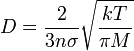
where the second factor is the mean free path and the square root (with Boltzmann's constant k) is the mean velocity of the particles.

In turbulent flows, the transport by eddy motion can be expressed as a grossly increased diffusion coefficient.

Quantum mechanics

Main article: Probability current

In quantum mechanics, particles of mass m in the quantum state ψ(r, t) have a probability density defined as

$\rho = \psi^* \psi = |\psi|^2. \,$

So the probability of finding a particle in a differential volume element d³r is

${\rm d}P = |\psi|^2 {\rm d}^3\mathbf{r}. \,$

Then the number of particles passing perpendicularly through unit area of a cross-section per unit time is the probability flux;

$\mathbf{J} = \frac{i \hbar}{2m} \left(\psi \nabla \psi^* - \psi^* \nabla \psi \right). \,$

This is sometimes referred to as the probability current or current density, or probability flux density.

Flux as a surface integral

The flux visualized. The rings show the surface boundaries. The red arrows stand for the flow of charges, fluid particles, subatomic particles, photons, etc. The number of arrows that pass through each ring is the flux.

General mathematical definition (surface integral)

As a mathematical concept, flux is represented by the surface integral of a vector field,

$\Phi_F=$${\scriptstyle A}$$\bold{F} \cdot {\rm d}\bold{A}$

where F is a vector field, and dA is the vector area of the surface A, directed as the surface normal,

The surface has to be orientable, i.e. two sides can be distinguished: the surface does not fold back onto itself. Also, the surface has to be actually oriented, i.e. we use a convention as to flowing which way is counted positive; flowing backward is then counted negative.

The surface normal is directed usually by the right-hand rule.

Conversely, one can consider the flux the more fundamental quantity and call the vector field the flux density.

Often a vector field is drawn by curves (field lines) following the "flow"; the magnitude of the vector field is then the line density, and the flux through a surface is the number of lines. Lines originate from areas of positive divergence (sources) and end at areas of negative divergence (sinks).

See also the image at right: the number of red arrows passing through a unit area is the flux density, the curve encircling the red arrows denotes the boundary of the surface, and the orientation of the arrows with respect to the surface denotes the sign of the inner product of the vector field with the surface normals.

If the surface encloses a 3D region, usually the surface is oriented such that the influx is counted positive; the opposite is the outflux.

The divergence theorem states that the net outflux through a closed surface, in other words the net outflux from a 3D region, is found by adding the local net outflow from each point in the region (which is expressed by the divergence).

If the surface is not closed, it has an oriented curve as boundary. Stokes' theorem states that the flux of the curl of a vector field is the line integral of the vector field over this boundary. This path integral is also called circulation, especially in fluid dynamics. Thus the curl is the circulation density.

We can apply the flux and these theorems to many disciplines in which we see currents, forces, etc., applied through areas.

Electromagnetism

To better understand the concept of flux in Electromagnetism, imagine a butterfly net. The amount of air moving through the net at any given instant in time is the flux. If the wind speed is high, then the flux through the net is large. If the net is made bigger, then the flux would be larger even though the wind speed is the same. For the most air to move through the net, the opening of the net must be facing the direction the wind is blowing. If the net opening is parallel to the wind, then no wind will be moving through the net. The simplist way to think of flux is "how much air goes through the net", where the air is a (velocity) field and the net is the boundray of an imaginary surface.

Electric flux

Two forms of electric flux are used, one for the E-field:

$\Phi_E=$${\scriptstyle A}$$\bold{E} \cdot {\rm d}\bold{A}$

and one for the D-field (called the electric displacement):

$\Phi_D=$${\scriptstyle A}$$\bold{D} \cdot {\rm d}\bold{A}$

This quantity arises in Gauss's law - which states that the flux of the electric field E out of a closed surface is proportional to the electric charge Q_A enclosed in the surface (independent of how that charge is distributed), the integral form is:

${\scriptstyle A}$$\bold{E} \cdot {\rm d}\bold{A} = Q_A$

where ε₀ is the permittivity of free space.

If one considers the flux of the electric field vector, E, for a tube near a point charge in the field the charge but not containing it with sides formed by lines tangent to the field, the flux for the sides is zero and there is an equal and opposite flux at both ends of the tube. This is a consequence of Gauss's Law applied to an inverse square field. The flux for any cross-sectional surface of the tube will be the same. The total flux for any surface surrounding a charge q is q/ε₀.

In free space the electric displacement is given by the constitutive relation D = ε₀ E, so for any bounding surface the D-field flux equals the charge Q_A within it. Here the expression "flux of" indicates a mathematical operation and, as can be seen, the result is not necessarily a "flow", since nothing actually flows along electric field lines.

Magnetic flux

The magnetic field is denoted by B, and magnetic flux is defined analagously:

$\Phi_B=$${\scriptstyle A}$$\bold{B} \cdot {\rm d}\bold{A}$

with the same notation above. The quantity arises in Faraday's law of induction, in integral form:

$\oint_C \mathbf{E} \cdot d \boldsymbol{\ell} = -\int_{\partial C} {\partial \mathbf{B}\over \partial t} \cdot {\rm d}\mathbf{s} = - \frac{{\rm d} \Phi_D}{ {\rm d} t}$

where dℓ is an infinitesimal vector line element of the closed curve C, with magnitude equal to the length of the infinitesimal line element, and direction given by the tangent to the curve C, with the sign determined by the integration direction.

The time-rate of change of the magnetic flux through a loop of wire is minus the electromotive force created in that wire. The direction is such that if current is allowed to pass through the wire, the electromotive force will cause a current which "opposes" the change in magnetic field by itself producing a magnetic field opposite to the change. This is the basis for inductors and many electric generators.

Poynting flux

Using this definition, the flux of the Poynting vector S over a specified surface is the rate at which electromagnetic energy flows through that surface, defined like before:

$\Phi_S=$${\scriptstyle A}$$\bold{S} \cdot {\rm d}\bold{A}$

The flux of the Poynting vector through a surface is the electromagnetic power, or energy per unit time, passing through that surface. This is commonly used in analysis of electromagnetic radiation, but has application to other electromagnetic systems as well.

Confusingly, the Poynting vector is sometimes called the power flux, which is an example of the first usage of flux, above. It has units of watts per square metre (W/m²).

Biology

In general, flux in biology relates to movement of a substance between compartments. There are several cases where the concept of flux is important.

• The movement of molecules across a membrane: in this case, flux is defined by the rate of diffusion or transport of a substance across a permeable membrane. Except in the case of active transport, net flux is directly proportional to the concentration difference across the membrane, the surface area of the membrane, and the membrane permeability constant.
• In ecology, flux is often considered at the ecosystem level - for instance, accurate determination of carbon fluxes using techniques like eddy covariance (at a regional and global level) is essential for modeling the causes and consequences of global warming.
• Metabolic flux refers to the rate of flow of metabolites along a metabolic pathway, or even through a single enzyme. A calculation may also be made of carbon (or other elements, e.g. nitrogen) flux. It is dependent on a number of factors, including: enzyme concentration; the concentration of precursor, product, and intermediate metabolites; post-translational modification of enzymes; and the presence of metabolic activators or repressors. Metabolic control analysis and flux balance analysis provide frameworks for understanding metabolic fluxes and their constraints.

See also

AB magnitude Explosively pumped flux compression generator Eddy covariance flux (aka, eddy correlation, eddy flux) Fast Flux Test Facility Fluence (flux for particle beams) Fluid dynamics Flux footprint Flux pinning Flux quantization Gauss's law Inverse-square law

Jansky unit, another way to represent flux density Latent heat flux Luminous flux Magnetic flux Magnetic flux quantum Neutron flux Poynting flux Poynting theorem Radiant flux Rapid single flux quantum Sound energy flux Volumetric flow rate

Further reading

• Stauffer, P.H. (2006). "Flux Flummoxed: A Proposal for Consistent Usage". Ground Water 44 (2): 125–128. DOI:10.1111/j.1745-6584.2006.00197.x. PMID 16556188.