Ch 3 - Using Statistical Analysis

• 3.0 - Chapter Introduction
• 3.1 - Identifying Situations For Use
• 3.2 - Measuring Central Tendency
• 3.3 - Measuring Dispersion
• 3.4 - Establishing A Confidence Interval
• 3.5 - Using Stratified Sampling
• 3.6 - Identifying Issues and Concerns

3.0 - Chapter Introduction

In this chapter, you will learn to use descriptive statistics to organize, summarize, analyze, and interpret data for contract pricing.

Categories of Statistics. Statistics is a science which involves collecting, organizing, summarizing, analyzing, and interpreting data in order to facilitate the decision-making process. These data can be facts, measurements, or observations. For example, the inflation rate for various commodity groups is a statistic which is very important in contract pricing. Statistics can be classified into two broad categories:

• Descriptive Statistics. Descriptive statistics include a large variety of methods for summarizing or describing a set of numbers. These methods may involve computational or graphical analysis. For example, price index numbers are one example of a descriptive statistic. The measures of central tendency and dispersion presented in this chapter are also descriptive statistics, because they describe the nature of the data collected.
• Inferential Statistics. Inferential or inductive statistics are methods of using a sample data taken from a statistical population to make actual decisions, predictions, and generalizations related to a problem of interest. For example, in contract pricing, we can use stratified sampling of a proposed bill of materials to infer the degree it is overpriced or under-priced.

Populations and Samples. The terms population and sample are used throughout any discussion of statistics.

• Population. A population is the set of all possible observations of a phenomenon with which we are concerned. For example, all the line items in a bill of materials would constitute a population. A numerical characteristic of a population is called a parameter.
• Sample. A sample is a subset of the population of interest that is selected in order to make some inference about the whole population. For example, a group of line items randomly selected from a bill of materials for analysis would constitute a sample. A numerical characteristic of a sample is called a statistic.

In contract pricing, you will most likely use statistics because you do not have complete knowledge of the population or you do not have the resources needed to examine the population data. Because most pricing applications involve the use of sample data, this chapter will concentrate on statistical analysis using sample data. If you are interested in learning about descriptive or inferential analysis of numerical population data, consult a college level statistics text.

Measure of Reliability. Since a sample contains only a portion of observations in the population, there is always a chance that our inference or generalization about the population will be inaccurate. Therefore, our inference should be accompanied by a measure of reliability. For example, let's assume that we are 90 percent sure that the average item in a bill of materials should cost 85 percent of what the contractor has proposed plus or minus 3 percent. The 3 percent is simply a boundary for our prediction error and it means there is a 90 percent probability that the error of our prediction is not likely to exceed 3 percent.

3.1 - Identifying Situations For Use

Situations for Use. Statistical analysis can be invaluable to you in:

• Developing Government objectives for contract prices based on historical values. Historical costs or prices are often used as a basis for prospective contract pricing. When several historical data points are available, you can use statistical analysis to evaluate the historical data in making estimates for the future. For example, you might estimate the production equipment set-up time based on average historical set-up times.
• Developing minimum and maximum price positions for negotiations. As you prepare your negotiation objective, you can also use statistical analysis to develop minimum and maximum positions through analysis of risk. For example, if you develop an objective of future production set-up time based on the average of historical experience, that average is a point estimate calculated from many observations. If all the historical observations are close to the point estimate, you should feel confident that actual set-up time will be close to the estimate. As the differences between the individual historical observations and the point estimate increase, the risk that the future value will be substantially different than the point estimate also increases. You can use statistical analysis to assess the cost risk involved and use that assessment in developing your minimum and maximum negotiation positions.
• Developing an estimate of risk for consideration in contract type selection. As described above, you can use statistical analysis to analyze contractor cost risk. In addition to using that analysis in developing your minimum and maximum negotiation positions you can use it in contract type selection. For example, if the risk is so large that a firm fixed-price providing reasonable protection to the contractor could also result in a wind-fall profit, you should consider an incentive or cost-reimbursement contract instead.
• Developing an estimate of risk for consideration in profit/fee analysis. An analysis of cost risk is also an important element in establishing contract profit/fee objectives. The greater the dispersion of historical cost data, the greater the risk in prospective contract pricing. As contractor cost risk increases, contract profit/fee should also increase.
• Streamlining the evaluation of a large quantity of data without sacrificing quality. Statistical sampling is particularly useful in the analysis of a large bill of materials. The stratified sampling techniques presented in this chapter allow you to:
  • Examine 100 percent of the items with the greatest potential for cost reduction; and
  • Use random sampling to assure that there is no general pattern of overpricing smaller value items.
  • The underlying assumption of random sampling is that a sample is representative of the population from which it is drawn.
  • If the sample is fairly priced, the entire stratum is assumed to be fairly priced; if the sample is overpriced, the entire stratum is assumed to be proportionately overpriced.

3.2 - Measuring Central Tendency

Measures of Central Tendency. You are about to prepare a solicitation for a product that your office has acquired several times before. Before you begin, you want to know what your office has historically paid for the product. You could rely exclusively on the last price paid, or you could collect data from the last several acquisitions. An array of data from several acquisitions will likely mean little without some statistical analysis.

To get a clearer picture of this array of data, you would likely want to calculate some measure of central tendency. A measure of central tendency is the central value around which data observations (e.g., historical prices) tend to cluster. It is the central value of the distribution. This section will examine calculation of the three most common and useful measures of central tendency:

• Arithmetic mean;
• Median; and
• Mode.

Calculating the Arithmetic Mean. The arithmetic mean (or simply the mean or average) is the measure of central tendency most commonly used in contract pricing. To calculate the mean, sum all observations in a set of data and divide by the total number of observations involved. The formula for this calculation is:

Where:

= Sample mean

S = Summation of all the variables that follow the symbol (e.g., S X represents the sum of all X values)

X = Value for an observation of the variable X

n = Total number of observations in the sample

For example: Suppose you are trying to determine the production lead time (PLT) for an electronic component using the following sample data:

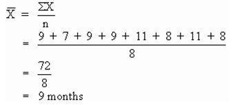
Calculating the Median. The median is the middle value of a data set when the observations are arrayed from the lowest to the highest (or from the highest to the lowest). If the data set contains an even number of observations, the median is the arithmetic mean of the two middle observations.

It is often used to measure central tendency when a few observations might pull the measure from the center of the remaining data. For example, average housing value in an area is commonly calculated using the median, because a few extremely high-priced homes could result in a mean that presents an overvalued picture of the average home price.

For the PLT example: You could array the data from lowest to highest:

Since there is an even number of observations, calculate median using the arithmetic mean of the two middle observations:

Calculating the Mode. The mode is the observed value that occurs most often in the data set (i.e. the value with the highest frequency).

It is often used to estimate which specific value is most likely to occur in the future. However, a data set may have more than one mode. A data set is described as:

• Unimodal if it has only one mode.
• Bimodal if it has two modes.
• Multimodal if it has more than two modes.

For the PLT example: The mode is nine, because nine occurs three times, once more than any other value.

3.3 - Measuring Dispersion

Measures of Dispersion. As described in the previous section, the mean is the measure of central tendency most commonly used in contract pricing. Though the mean for a data set is a value around which the other values tend to cluster, it conveys no indication of the closeness of the clustering (that is, the dispersion). All observations could be close to the mean or far away.

If you want an indication of how closely these other values are clustered around the mean, you must look beyond measures of central tendency to measures of dispersion. This section will examine:

• Several measures of absolute dispersion commonly used to describe the variation within a data set -- the range, mean absolute deviation, variance, and standard deviation.
• One measure of relative dispersion-- the coefficient of variation.

Assume that you have the following scrap rate data for two contractor departments:

The mean scrap rate for both departments is the same -- 5 percent. However, the monthly scrap rates in Department B show less variation (dispersion) around the mean. As a result, you would probably feel more comfortable forecasting a scrap rate of 5 percent for Department B than you would for Department A.

Differences in dispersion will not always be so obvious. The remainder of this section will demonstrate how you can quantify dispersion using the five measures identified above.

Calculating the Range. Probably the quickest and easiest measure of dispersion to calculate is the range. The range of a set of data is the difference between the highest and lowest observed values. The higher the range, the greater the amount of variation in a data set.

R = H - L

Where:

R = Range

H = Highest observed value in the data set

L = Lowest observed value in the data set

Calculating the Range for the Scrap-Rate Example. By comparing the range for Department A scrap-rate data with the range for Department B, you can easily determine that the historical data from Department A shows greater dispersion.

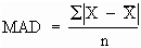
Mean Absolute Deviation. The mean absolute deviation (MAD) is the average absolute difference between the observed values and the arithmetic mean (average) for all values in the data set.

If you subtracted the mean from each observation, some answers would be positive and some negative. The sum of all the deviations (differences) will always be zero. That tells you nothing about how far the average observation is from the mean. To make that computation, you can use the absolute difference between each observation and the mean. An absolute difference is the difference without consideration of sign and all absolute values are written as positive numbers. If the average is eight and the observed value is six, the calculated difference is a negative two (6 - 8 = -2), but the absolute difference would be two (without the negative sign).

Note: Absolute values are identified using a vertical line before and after the value (e.g., |X| identifies the absolute value of X).

To compute the MAD, use the following 5-step process:

Step 1. Calculate the arithmetic mean of the data set.

Step 2. Calculate the deviation (difference) between each observation and the mean of the data set.

Step 3. Convert each deviation to its absolute value (i.e., its value without considering the sign of the deviation).

Step 4. Sum the absolute deviations.

Step 5. Divide the total absolute deviation by the number of observations in the data set.

Calculating the Mean Absolute Deviation for the Scrap-Rate Example. We can use the 5-step process described above to calculate the scrap-rate MAD values for Departments A and B of the scrap-rate example.

Calculate the MAD for Department A:

Step 1. Calculate the arithmetic mean of the data set. We have already calculated the mean rate for Department A of the scrap-rate example -- .05.

Step 2. Calculate the deviation (difference) between each observation and the mean of the data set .

Step 3. Convert each deviation to its absolute value .

Step 4. Sum the absolute deviations .

Step 5. Divide the total absolute deviation by the number of observations in the data set.

Calculate the MAD for Department B:

Step 1. Calculate the arithmetic mean of the data set. We have also calculated the mean rate for Department B of the scrap-rate example -- .05.

Steps 2 - 4. Calculate the deviation between each observation and the mean of the data set; convert the deviation to its absolute value; and sum the absolute deviations. The following table demonstrates the three steps required to calculate the total absolute deviation for Department B:

Step 5. Divide the total absolute deviation by the number of observations in the data set.

Compare MAD values for Department A and Department B:

The MAD for Department A is .014; the MAD for Department B is .002. Note that the MAD for Department B is much smaller than the MAD for Department A. This comparison once again confirms that there is less dispersion in the observations from Department B.

Calculating the Variance. Variance is one of the two most popular measures of dispersion (the other is the standard deviation which is described below). The variance of a sample is the average of the squared deviations between each observation and the mean.

However, statisticians have determined when you have a relatively small sample, you can get a better estimate of the true population variance if you calculate variance by dividing the sum of the squared deviations by n - 1, instead of n.

The term, n - 1, is known as the number of degrees of freedom that can be used to estimate population variance.

This adjustment is necessary, because samples are usually more alike than the populations from which they are taken. Without this adjustment, the sample variance is likely to underestimate the true variation in the population. Division by n - 1 in a sense artificially inflates the sample variance but in so doing, it makes the sample variance a better estimator of the population variance. As the sample size increases, the relative affect of this adjustment decreases (e.g., dividing by four rather than five will have a greater affect on the quotient than dividing by 29 instead of 30).

To compute the variance, use this 5-step process:

Step 1. Calculate the arithmetic mean of the data set.

Step 2. Calculate the deviation (difference) between each observation and the mean of the data set.

Step 3. Square each deviation.

Step 4. Sum the squared deviations.

Step 5. Divide the sum of the squared deviations by n-1.

Calculate the variance for Department A:

Step 1. Calculate the arithmetic mean of the data set. We have already calculated the mean rate for Department A of the scrap-rate example -- .05.

Step 2. Calculate the deviation (difference) between each observation and the mean of the data set . The deviations for Department A are the same as we calculated in calculating the mean absolute deviation.

Step 3. Square each deviation .

Step 4. Sum the total absolute deviations .

Step 5. Divide the sum of the squared deviations by n-1.

Calculate the variance for Department B

Step 1. Calculate the arithmetic mean of the data set. We have also calculated the mean rate for Department B of the scrap-rate example -- .05.

Steps 2 - 4. Calculate the deviation between each observation and the mean of the data set; convert the deviation to its absolute value; and sum the absolute deviations. The following table demonstrates the three steps required to calculate the total absolute deviation for Department B:

Step 5. Divide the sum of the squared deviations by n-1.

Compare variances for Department A and Department B:

The variance for Department A is .000245; the variance for Department B is .000004. Once again, the variance comparison confirms that there is less dispersion in the observations from Department B.

Concerns About Using the Variance as a Measure of Dispersion. There are two concerns commonly raised about using the variance as a measure of dispersion:

• As the deviations between the observations and the mean grow, the variation grows much faster, because all the deviations are squared in variance calculation.
• The variance is in a different denomination than the values of the data set. For example, if the basic values are measured in feet, the variance is measured in square feet; if the basic values are measured in terms of dollars, the variance is measured in terms of "square dollars."

Calculating the Standard Deviation. You can eliminate these two common concerns by using the standard deviation -- the square root of the variance.

For example: You can calculate the standard deviation for Departments A and B of the scrap-rate example:

The standard deviation for Departments A and B of the scrap-rate example yields a standard deviation of .015652 for Department A, and .002000 for Department B.

Note: Both the variance and the standard deviation give increasing weight to observations that are further away from the mean. Because all values are squared, a single observation that is far from the mean can substantially affect both the variance and the standard deviation.

Empirical Rule. The standard deviation has one characteristic that makes it extremely valuable in statistical analysis. In a distribution of observations that is approximately symmetrical (normal):

• The interval ± 1S includes approximately 68 percent of the total observations in the population.
• The interval ± 2S includes approximately 95 percent of the total observations in the population.
• The interval ± 3S includes approximately 99.7 percent of the total observations in the population.

This relationship is actually a finding based on analysis of the normal distribution (bell shaped curve) that will be presented later in the chapter.

Coefficient of Variation. Thus far we have only compared two samples with equal means. In that situation, the smaller the standard deviation, the smaller the relative dispersion in the sample observations. However, that is not necessarily true when the means of two samples are not equal.

If the means are not equal, you need a measure of relative dispersion. The coefficient of variation (CV) is such a measure.

For example: Which of the following samples has more relative variation?

Calculate CV for Sample C:

Calculate CV for Sample D:

Compare the two CV values:

Even though the standard deviation for Sample D is twice as large as the standard deviation for Sample C, the CV values demonstrate that Sample D exhibits less relative variation. This is true because the mean for Sample D is so much larger than the mean for Sample C.

Note: We could calculate CV for the scrap-rate example, but such a calculation is not necessary because the means of the two samples are equal.

3.4 Establishing a Confidence Interval

Confidence Interval. Each time you take a sample from a population of values you can calculate a mean and a standard deviation. Even if all the samples are the same size and taken using the same random procedures, it is unlikely that every sample will have the same mean and standard deviation. However, if you could collect all possible samples from the normally distributed population and calculate the mean value for all the sample means, the result would be equal to the population mean. In statistical terminology, the mean of the sampling distribution is equal to the population mean.

You can combine the sample mean and sample standard deviation with an understanding of the shape of distribution of sample means to develop a confidence interval -- a probability statement about an interval which is likely to contain the true population mean.

For example: Suppose that you are preparing a solicitation for an indefinite-quantity transmission overhaul contract to support a fleet of 300 light utility trucks. You believe that you can develop an accurate estimate of the number of transmissions that will require a major overhaul during the contract period, if you can determine the date of the last major overhaul for each vehicle transmission and estimate the period between overhauls. You select a simple random sample (without replacement) of 25 vehicle maintenance records from the 300 fleet vehicle maintenance records. Analyzing the sample, you find that the mean time between overhauls is 38 months and the sample standard deviation (S) is 4 months. Based on this analysis, your point estimate of the average transmission life for all vehicles in the fleet (the population mean) is 38 months. But you want to establish reasonable estimates of the minimum and maximum number of repairs that will be required during the contract period. You want to be able to state that you are 90% confident that the average fleet transmission life is within a defined range (e.g., between 36 and 40 months).

To make this type of statement, you need to establish a confidence interval. You can establish a confidence interval using the sample mean, the standard error of the mean, and an understanding of the normal probability distribution and the t distribution.

Standard Error of the Mean. If the population is normally distributed, the standard error of the mean is equal to the population standard deviation divided by the square root of sample size. Since we normally do not know the population standard deviation, we normally use the sample standard deviation to estimate the population standard deviation.

Though the population mean and the population standard deviation are not normally known, we assume that cost or pricing information is normally distributed. This is a critical assumption because it allows us to construct confidence intervals (negotiation ranges) around point estimates (Government objectives).

Calculate the Standard Error of the Mean for the Transmission Example.

Remember that: S = 4 months

n = 25 vehicle maintenance records

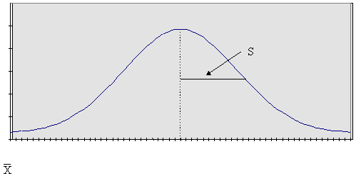
Normal Probability Distribution. The normal probability distribution is the most commonly used continuous distribution. Because of its unique properties, it applies to many situations in which it is necessary to make inferences about a population by taking samples. It is a close approximation of the distribution of such things as human characteristics (e.g., height, weight, and intelligence) and the output of manufacturing processes (e.g., fabrication and assembly). The normal probability distribution provides the probability of a continuous random variable, and has the following characteristics:

• It is a symmetrical (i.e., the mean, median, and mode are all equal) distribution and half of the possible outcomes are on each side of the mean.
• The total area under the normal curve is equal to 1.00. In other words, there is a 100 percent probability that the possible observations drawn from the population will be covered by the normal curve.
• It is an asymptotic distribution (the tails approach the horizontal axis but never touch it).
• It is represented by a smooth, unimodal, bell-shaped curve, usually called a "normal probability density function" or "normal curve."
• It can be defined by two characteristics-the mean and the standard deviation. (See the figure below.)

NORMAL CURVE

Conditions for Using the Normal Distribution. You can use the normal curve to construct confidence intervals around a sample mean when you know the population mean and standard deviation.

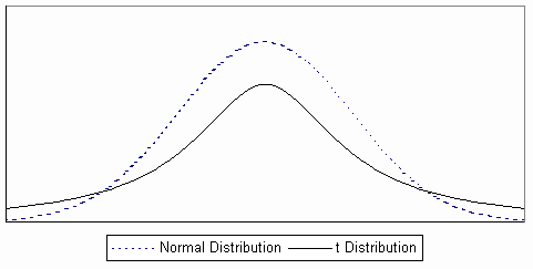
t Distribution. In contract pricing, the conditions for using the normal curve are rarely met. As a result, you will normally need to use a variation of the normal distribution called the "t-distribution."

The t distribution has the following characteristics:

• It is symmetrical, like the normal distribution, but it is a flatter distribution (higher in the tails).
• Whereas a normal distribution is defined by the mean and the standard deviation, the t distribution is defined by degrees of freedom.
• There is a different t distribution for each sample size.
• As the sample size increases, the shape of the t distribution approaches the shape of the normal distribution.

t Distribution

Relationship Between Confidence Level and Significance Level.

Confidence Level. The term confidence level refers to the confidence that you have that a particular interval includes the population mean. In general terms, a confidence interval for a population mean when the population standard deviation is unknown and n < 30 can be constructed as follows:

Where:

t = t Table value based on sample size and the significance level

= Standard error of the mean

Significance Level. ) The significance level is equal to 1.00 minus the confidence level. For example if the confidence level is 95 percent, the significance level is 5 percent; if the confidence level is 90 percent, the significance level is 10 percent. The significance level is, then, the area outside the interval which is likely to contain the population mean.

The figure below depicts a 90 percent confidence interval. Note that the significance level is 10 percent -- a 5 percent risk that the population mean is greater than the confidence interval plus a 5 percent risk that the mean is less than the confidence interval.

90 Percent Confidence Interval

Setting the Significance Level. When you set the significance level, you must determine the amount of risk you are willing to accept that the confidence interval does not include the true population mean. As the amount risk that you are willing to accept decreases, the confidence interval will increase. In other words, to be more sure that the true population mean in included is the interval, you must widen the interval.

Your tolerance for risk may vary from situation to situation, but for most pricing decisions, a significance level of .10 is appropriate.

Steps for Determining the Appropriate t Value for Confidence Interval Construction. After you have taken a random sample, calculated the sample mean and the standard error of the mean, you need only a value of t to construct a confidence interval. To obtain the appropriate t value, use the following steps:

Step 1. Determine your desired significance level. As stated above, for most contract pricing situations, you will find a significance level of .10 appropriate. That will provide a confidence level of .90 (1.00 - .10 = .90).

Step 2. Determine the degrees of freedom. Degrees of freedom (df) are the sample size minus one (n - 1).

Step 3. Determine the t value from the t Table. Find the t value at the intersection of the df row and the .10 column.

Constructing a Confidence Interval for the Transmission Overhaul Example. Recall the transmission overhaul example, where you wanted to estimate the useful life of transmissions of a fleet of 300 light utility trucks. We took a random sample of size n = 25 and calculated the following:

Where:

= 38 months

S = 4 months

= .8 months

Assume that you want to construct a 90% confidence interval for the population mean (the actual average useful life of the transmissions). You have all the values that you need to substitute into the formula for confidence interval except the t value. To determine the t value for a confidence interval, use the following steps:

Determine the appropriate t value:

Step 1. Determine the significance level. Use the significance level of .10.

Step 2. Determine the degrees of freedom.

Step 3. Determine the t value from the t Table. Find the t value at the intersection of the df = 24 row and the .10 column. The following table is an excerpt of the t Table:

Reading from the table, the appropriate t value is 1.711.

Use the t Value and Other Data to Construct Confidence Interval:

The confidence interval for the true population mean (the actual average useful life of the transmissions) would be:

38 ± 1.711 (.8)

38 ± 1.37 (rounded from 1.3688)

Confidence interval for the population mean (µ): 36.63 < µ < 39.37

That is, you would be 90 percent confident that the average useful life of the transmissions is between 36.63 and 39.37 months.

3.5 Using Stratified Sampling

Stratified Sampling Applications in Contract Pricing. You should consider using sampling when you have a large amount of data and limited time to conduct your analysis. While there are many different methods of sampling, stratified sampling is usually the most efficient and effective method of sampling for cost/price analysis. Using stratified sampling allows you to concentrate your efforts on the items with the greatest potential for cost/price reduction while using random sampling procedures to identify any general pattern of overpricing of smaller value items.

The most common contract pricing use of stratified sampling is analysis of detailed material cost proposals. Often hundreds, even thousands, of material items are purchased to support production of items and systems to meet Government requirements. To analyze the quantity requirements and unit prices for each item would be extremely time consuming and expensive. Effective review is essential, because often more than 50 percent of the contract price is in material items. The overall environment is custom made for the use of stratified sampling.

Steps in Stratified Sampling. In stratified sampling, the components of the proposed cost (e.g., a bill of materials) to be analyzed are divided into two or more groups or strata for analysis. One group or stratum is typically identified for 100 percent review and the remaining strata are analyzed on a sample basis. Use the following steps to develop a negotiation position based on stratified sampling:

Step 1. Identify a stratum of items that merit 100 percent analysis. Normally, these are high-value items that merit the cost of 100 percent analysis. However, this stratum may also include items identified as high-risk for other reasons (e.g., a contractor history of overpricing).

Step 2. Group the remaining items into one or more stratum for analysis. The number of additional strata necessary for analysis will depend on several factors:

• If the remaining items are relatively similar in price and other characteristics (e.g., industry, type of source, type of product), only one additional stratum may be required.
• If the remaining items are substantially different in price or other characteristics, more than one stratum may be required. For example, you might create one stratum for items with a total cost of $5,001 to $20,000 and another stratum for all items with a total cost of $5,000 or less.
• If you use a sampling procedure that increases the probability of selecting larger dollar items (such as the dollar unit sampling procedure available in E-Z-Quant), the need for more than one stratum may be reduced.

Step 3. Determine the number of items to be sampled in each stratum. You must analyze all items in the strata requiring 100 percent analysis. For all other strata, you must determine how many items you will sample. You should consider several factors in determining sample size. The primary ones are variability, desired confidence, and the total count of items in the stratum. Use statistical tables or computer programs to determine the proper sample size for each stratum.

Step 4. Select items for analysis. In the strata requiring random sampling, each item in the stratum must have an equal chance of being selected and each item must only be selected once for analysis. Assign each item in the population a sequential number (e.g., 1, 2, 3; or 1001, 1002, 1003). Use a table of random numbers or computer generated random numbers to identify the item numbers to be included in the sample.

Step 5. Analyze all items identified for analysis, summing recommended costs or prices for the 100 percent analysis stratum and developing a decrement factor for any stratum being randomly sampled. In the stratum requiring 100 percent analysis, you can apply any recommended price reductions directly to the items involved. In any stratum where you use random sampling, you must apply any recommended price reductions to all items in the stratum.

• Analyze the proposed cost or price of each sampled item.
• Develop a "should pay" cost or price for the item. You must do this for every item in the sample, regardless of difficulty, to provide statistical integrity to the results. If you cannot develop a position on a sampled item because offeror data for the item is plagued by excessive misrepresentations or errors, you might have to discontinue your analysis and return the proposal to the offeror for correction and update.
• Determine the average percentage by which should pay prices for the sampled items differ from proposed prices. This percentage is the decrement factor.

(There are a number of techniques for determining the "average" percentage which will produce different results. For example, you could (1) determine the percentage by which each should pay price differs from each proposed price, (2) sum the percentages, and (3) divide by the total number of items in the sample. This technique gives equal weight to all sampled items in establishing the decrement factor. Or you could (1) total proposed prices for all sampled items, (2) total the dollar differences between should pay and proposed prices, and (3) divide the latter total by the former total. This technique gives more weight to the higher priced sampled items in establishing the decrement factor.)

• Calculate the confidence interval for the decrement factor.

Step 6. Apply the decrement factor to the total proposed cost of all items in the stratum. The resulting dollar figure is your prenegotiation position for the stratum. Similarly, use confidence intervals to develop the negotiation range.

Step 7. Sum the prenegotiation positions for all strata to establish your overall position on the cost category.

Stratified Sampling Example. Assume you must analyze a cost estimate that includes 1,000 material line items with a total cost of $2,494,500. You calculate that you must analyze a simple random sample of 50 line items.

Step 1. Identify a stratum of items that merit 100 percent analysis. You want to identify items that merit 100 percent analysis because of their relatively high cost. To do this, you prepare a list of the 1,000 line items organized from highest extended cost to lowest extended. The top six items on this list look like this:

Item 1: $675,000

Item 2: $546,500

Item 3: $274,200

Item 4: $156,800

Item 5: $101,300

Item 6: $ 26,705

Note that the top five items $1,753,800 (about 70 percent of the total material cost). You will commonly find that a few items account for a large portion of proposed material cost. Also note that there is a major drop from $101,300 to $26,705. This is also common. Normally, you should look for such break points in planning for analysis. By analyzing Items 1 to 5, you will consider 70 percent of proposed contract cost. You can use random sampling procedures to identify pricing trends in the remaining 30 percent.

Step 2. Group the remaining items into one or more stratum for analysis. A single random sampling stratum is normally adequate unless there is a very broad range of prices requiring analysis. This typically only occurs with multimillion dollar proposals. Here, the extended prices for the items identified for random sampling range from $5.00 to $26,705. While this is a wide range, the dollars involved seem to indicate that a single random sampling strata will be adequate.

Step 3. Determine the number of items to be sampled in each stratum. Based on the dollars and the time available, you determine to sample a total of 20 items from the remaining 995 on the bill of materials.

Step 4. Select items for analysis.

• One way that you could select items for analysis would be putting 1,000 sheets of paper, one for each line item, into a large vat, mix them thoroughly, and select 20 slips of paper from the vat. If the slips of paper were thoroughly mixed, you would identify a simple random sample.
• A less cumbersome method would be to use a random number table (such as the example below) or a computer program to pick a simple random sample. A random number is one in which the digits 0 through 9 appear in no particular pattern and each digit has an equal probability (1/10) of occurring.

• The number of digits in each random number should be greater than or equal to the number of digits we have assigned to any element in the population.
• To sample a population of 995 items, numbered 1 to 995, random numbers must have at least three digits. Since you are dealing with three digit numbers, you only need to use the first three digits of any random number that includes four or more digits.
• Using a random number table below:
  • You could start at any point in the table. However, it is customary to select a start point at random. Assume that you start at Row 2, Column 3. The first number is 365; hence the first line item in our sample would be the item identified as 365.
  • Proceed sequentially until all 20 sample line items have been selected. The second number is 265, the third 570, etc. When you get to the end of the table you would go to Row 1, Column 4.

Step 5. Analyze all items identified for analysis summing recommended costs or prices for the 100 percent analysis stratum and developing a decrement factor for any stratum being randomly sampled.

Results of 100 Percent Analysis. Use of the 100 percent analysis is straight forward. In this example, the offeror proposed a total of $1,753,800 for 5 line items of material. An analysis of these items found that the unit cost estimates were based on smaller quantities than required for the contract. When the full requirement was used, the total cost for those five items decreased to $1,648,600. Since the analysis considered all items in the stratum, you simply need to use the findings in objective development.

Random Sample Results. The random sample included 20 items with an estimated cost of $75,000. Analysis finds that the cost of the sampled items should be only 98 percent of the amount proposed. However, the confidence interval indicates that costs may range from 96 to 100 percent of the costs proposed.

Step 6. Apply the decrement factor to the total proposed cost of all items in the stratum.

Results of 100 Percent Analysis. There is no need to apply a decrement factor to these items because the recommended cost of $1,648,600 resulted from analysis of all items in this stratum.

Random Sample Results. The assumption is that the sample is representative of the entire population. If the sample is overpriced, the entire population of is similarly overpriced. As a result the recommended cost objective would be $725,886, or 98 percent of the proposed $740,700. However, the confidence interval would be $711,072 ( 96 percent of $740,700) to $740,700 (100 percent of $740,700).

Step 7. Sum the prenegotiation positions for all strata to establish your overall position on the cost category.

Point Estimate. The total point estimate results from the 100 percent and random sample analyses would be $2,374,486 ($1,648,600 + $725,886).

Confidence Interval: The confidence interval would run from $2,359,672 ($1,648,600 + $711,072) to $2,389,300 ($1,648,600 + $740,700). Note that the position on the stratum subject to 100 percent analysis would not change.

3.6 Identifying Issues and Concerns

Questions to Consider in Analysis. As you perform price or cost analysis, consider the issues and concerns identified in this section, whenever you use statistical analysis.

• Are the statistics representative of the current contracting situation?

Whenever historical information is used to make an estimate of future contract performance costs, assure that the history is representative of the circumstances that the contractor will face during contract performance.

• Have you considered the confidence interval in developing a range of reasonable costs?

Whenever sampling procedures are used, different samples will normally result in different estimates concerning contractor costs. Assure that you consider the confidence interval in making your projections of future costs. Remember that there is a range of reasonable costs and the confidence interval will assist you in better defining that range.

• Is the confidence interval so large as to render the point estimate meaningless as a negotiation tool?

If the confidence interval is very large (relative to the point estimate), you should consider increasing the sample size or other means to reduce the risk involved.

• Is your analysis, including any sample analysis, based on current, accurate, and complete information?

A perfect analysis of information that is not current accurate and complete will likely not provide the best possible estimates of future contract costs.

• Do the items with questioned pricing have anything in common?

If items with questioned pricing are related, consider collecting them into a separate stratum for analysis. For example, you might find that a large number of pricing questions are related to quotes from a single subcontractor. Consider removing all items provided by that subcontractor from existing strata for separate analysis