February 2016
Note: Prior to download of the materials on this page, the Center for Innovative Finance Support will collect minimal contact information in order to notify you when materials are updated.
Download FAQs (PDF)
The Federal Highway Administration (FHWA)'s Center for Innovative Finance Support (formerly Innovative Program Delivery) compiled Frequently Asked Questions (FAQs) throughout the development and testing of the P3-VALUE 2.0 analytical tool. These FAQs supplement the User Guide and supporting materials (on risk assessment, value for money, benefit-cost analysis and P3 project financing) in providing technical assistance to tool users.
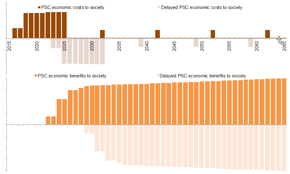
In the VfM analysis, the PSC is compared to the P3 in order to determine the fiscal impact on the Agency of P3 procurement. A key requirement for a VfM analysis to be valid is that the PSC and the P3 are implemented in a similar timeframe. For the PDBCA, there is no such requirement. Under PDBCA, a delayed project can be compared to an accelerated project without any conceptual challenges. The time delay in implementing the project would be estimated based on the budgetary and/or debt capacity of the Agency, and when sufficient funds might be available to begin and complete implementation of the project. The Delayed PSC has the exact same characteristics as the PSC, with only one exception: the start date of the project. If, for example, due to fiscal constraints an Agency can only afford to start building a project in 2025 instead of 2018, both the incurred costs as well as the benefits accruing to society will be delayed. Asset quality and value at handback therefore may be different as well. Depending on the exact profile of costs and benefits over time, accelerating a project may result in lower or higher net benefits to society.
The field "private procurement costs (costs of winning bid)" should include an estimate of the costs incurred by the winning bidder in preparing a bid and negotiating an agreement. If losing bidders receive any form of compensation, the cost is borne by the public agency and included in the field of "public procurement costs".
The field "private procurement costs (cost of non-compensated bids)" should include the procurement costs incurred by losing bidders that are not compensated by the public procuring agency.
The extent to which various costs are transferred to a P3 concessionaire depend on the presumed structure of the contract, project requirements, and risk sharing and allocation. The public agency can be responsible for preliminary design, right-of-way, and project oversight, but shift all engineering and construction responsibilities to the P3 concessionaire. The percentage transferred cost reflects the cost allocation between the public agency and P3 concessionaire. If separate cost estimates are available for P3 concessionaire and public agency respectively, the percentage of transferred costs can accordingly be set at 100% or 0%.
P3 projects may result in cost efficiencies by bundling different stages of project delivery under one contract and creating incentives to better manage the project's life cycle costs. However, there are no definitive studies regarding the cost efficiency of P3s in the United States. In studies where public agencies have compared P3 and conventional delivery options they have typically assumed cost efficiencies ranging from 0 to 15 percent. As the tool does not separately account for the cost impact of time efficiency in project delivery, this input should also include the impacts on cost reduction caused by time efficiency.
A comprehensive VfM analysis or PDBCA should not only consider what happens to the facility under different delivery models during the operations period but also what may happen thereafter. Therefore, the analysis period should at least cover the proposed concession period but should also take into consideration the residual value of the facility at handback. If appropriate handback provisions are included in the P3 agreement, the remaining useful life of the facility under conventional procurement may be assumed to be the same as under a P3 delivery at the end of the concession period.
P3-VALUE 2.0 can accommodate a variation in residual value of the facility under various delivery models. In order to take this variation into consideration, the user must determine the cost associated with bringing the facility back to the specified standards for each delivery model. By including these costs in the VfM analysis and PDBCA, the user can make a fair comparison of the different delivery models while allowing for variations in residual value of the facility.
In P3-VALUE 2.0 major maintenance costs are differentiated from operations and maintenance costs in that major maintenance costs are costs that occur on a periodic basis of multiple years (e.g., every 10 years) whereas operations and maintenance costs are assumed to occur on an annual basis. Major maintenance covers preservation activities that typically increase strength and extend facility service life in addition to restoring serviceability. For example, structural overlay and rehabilitation can be performed every 10-12 years. Routine maintenance is performed primarily to ensure or restore the function of the existing system.
Preconstruction and construction costs can be expressed in either in Year of Expenditure (YOE) or base year dollars. The tool applies "Indexation rate - Construction" to adjust base year dollars to YOE dollars. If preconstruction and construction costs are in YOE dollars, the field "Indexation rate - Construction" should be set to zero. Otherwise, a positive indexation rate should be used to reflect cost inflation during the pre-construction or construction period.
The various indexation rates can be used to account for the inflation of costs or payments during different periods of project delivery. Generally, costs and payments are expressed in base year dollars, and indexation rates are used to estimate Year of Expenditure (YOE) costs and payments. The base year is defined in the field "Indexation base year". The indexation rate for an availability payment can be used to model changes in the annual availability payment over the period of the concession. If a portion of the availability payment increases over the years of the concession term, the Indexation rate for availability payment should be adjusted accordingly. For example, if 20% of the availability payment is inflated at CPI of 2.5% per year, the indexation rate for availability is set to 0.5%.
Users are expected to provide No Build annual O&M costs (in thousands of dollars per year), which are used to calculate the O&M cost savings achieved by doing the project. The No Build annual O&M amount should include all operational costs that will not have to be incurred if the project is undertaken, including any contributions towards major maintenance.
The Delayed PSC has the exact same characteristics as the PSC, with only one exception: the start date of the project. If, for example, due to fiscal constraints an Agency can only afford to start building a project in 2025 instead of 2018, both the incurred costs as well as the benefits accruing to society will be delayed as can be seen in the figure below.
Comparison of economic costs & benefits between Delayed PSC and PSC

View larger version of comparison chart
The tool cannot easily model this scenario. The best approximation of this scenario may be a unidirectional three lanes alternative. The user needs to change the field "Number of directions in bidirectional traffic" to 1 in cell F109 in the "InpTiming&Cost" sheet. All other inputs must be calibrated carefully to reflect the traffic pattern in this scenario. It may be possible to conduct two separate analyses, one for each direction of travel, and combine the results.
Users are expected to provide a traffic sensitivity factor, which determines what share of the growth in P50 (or most likely) traffic will be considered in the PDBCA module. This factor is applied in order to capture the uncertainty in traffic projections. The factor is a percentage (less or more than 100%) of the P50 (or equivalent) traffic growth above the base year traffic and hence lowers or increases the traffic projections to be considered in the PDBCA sensitivity analysis. If, for example, daily traffic growth forecasted is 15,000 vehicles above base year traffic under P50 and the Agency believes that the traffic growth may possibly be about 20% above or below that forecast, the appropriate traffic sensitivity factors to be used would be 80% and 120%. In that case, the BCA module would be re-run with growth in traffic of 12,000 vehicles per day and 18,000 vehicles per day, in order to calculate the various societal costs and benefits and check whether the economic justification for the project and project delivery still holds. Note that the same factor is applied to both No Build and Build traffic growth forecasts.
In short, no, the total number of unidirectional peak and off peak hours do not need to equal 24 hours. The model requires users to input only the number of hours with significant traffic in order to ensure that off-peak congested speed is representative of real world conditions. For example, the amount of traffic carried by a roadway between 12:00 AM and 6:00 AM may be insignificant and in that case would not need to be included.
The tool calculates speeds for each year in the analysis period for the various delivery models. These speeds are used to compute travel time costs, incident delays, O&M-related travel delays, construction-related travel delays, non-fuel costs, fuel costs, and emissions costs. Capacities for peak, off-peak, and weekends are calculated using inputs from InpTraffic&Toll. Then vehicle volume/capacity for peak, off-peak, and weekends are calculated using traffic volumes from the Traffic sheet and capacities calculated in the above step. Speeds for peak, off-peak, and weekends are then calculated using volume delay function (VDF) parameters, free flow speeds from the InpTraffic&Toll sheet, and the V/C ratios calculated above. Delays due to construction, O&M activities, and incidents are also calculated. The concept guide (Chapter 5 in Part II of the Guide to P3-VALUE) explains the procedures in detail.
The users of P3-VALUE 2.0 must provide traffic projections for both the No Build and Build alternatives. Typically, these projections will be generated using a travel demand model. The difference between the No Build and Build traffic projections is induced traffic. These induced traffic projections are then used in the model to calculate the costs and benefits to society of induced traffic.
First, the No Build scenario is only used for the benefit cost analysis and has not impact on the financial value for money analysis.P3-VALUE 2.0 has certain limitations with regard to the type of projects it can analyze for the BCA analysis. For example, there is only one lane type and associated traffic input for the No Build. If the No Build contains both high occupancy vehicle (HOV) lanes and general purpose lanes (GPL), the user would need to combine both types of traffic into a single input. While the combined traffic volumes can be directly input, the vehicle occupancy for the No Build would need to be adjusted to represent both sets of lanes. In addition, HOV lanes and the GPLs may in reality have different congested speeds. Since a single Volume Delay Function (VDF) would be applied to the combined traffic, the estimated congested speeds will not reflect actual conditions. The VDF will overestimate the speed of GPL traffic and underestimate the speed of HOV traffic. Therefore, use of P3-VALUE 2.0 for this type of project will not provide an accurate representation of congestion delays in the No Build scenario.
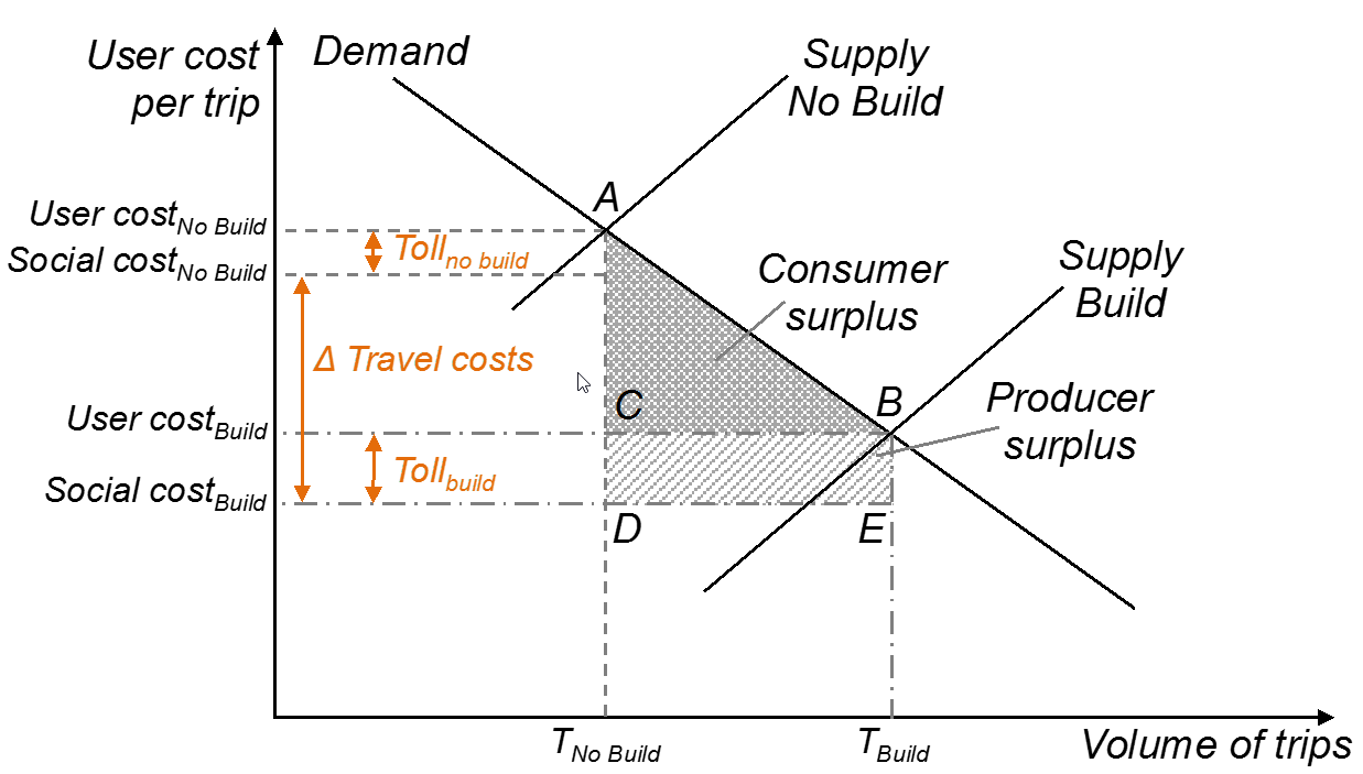
Second, tolls are considered to be a transfer payment and should not be included in calculating the benefits to existing users. For existing traffic, the introduction of tolls or change in toll levels between the No Build and Build alternatives does not modify the calculation of societal benefits. To determine the societal benefits of a facility expansion for existing traffic, the social costs of travel (i.e., excluding tolls which are transfers) for each existing user before and after the expansion are evaluated. The difference in travel costs multiplied by the number of existing users is the net benefit to society of the facility enhancement. For induced traffic, the rule of half can be used to calculate the societal costs and benefits if both the No Build and Build alternatives are not tolled. However, if the road is tolled in the Build or even in the No Build alternative, the rule of half - by itself can no longer be applied as the shape under the demand curve that represents the net benefits to society now has both a triangular consumer surplus and a rectangular producer surplus, as can be seen in the figure below. The producer surplus is equal to the toll level under the Build alternative multiplied with the induced traffic (CBDE in the figure below), and the consumer surplus calculation includes the consideration of tolls borne by users under both the Build and the No Build cases.
Effect of toll on consumer surplus and producer surplus
View larger version of the above graph
Project delivery benefit cost analysis evaluates P3 delivery from the societal perspective. Project capital costs, regardless of funding sources, will be included in the PDBCA analysis. A public agency may produce an agency specific PDBCA by reducing costs reimbursed by the federal government, especially in the case of discretionary grants. For example, if an agency receives federal discretionary grant funding to cover 20% of project capital costs, project costs can be reduced by 20% accordingly. However, assuming that the same amount of federal subsidy is available under both P3 and conventional delivery, the treatment of federal subsidies in the analysis should have not impact on the results of the comparison between delivery methods.
The user should enter the total combined amount of the milestone payments in the appropriate cell in the InpFin sheet. In the InpSeries sheet the user can then distribute that amount to the appropriate cash flow periods.
The model indeed does not explicitly contain this functionality. However, availability payments can be included in toll-based payment project by spreading a milestone payment out over time (e.g. 2.5% per year for 40 years).
P3 projects typically have complex financing structures, potentially involving a large number of debt and equity instruments. The P3-VALUE 2.0 tool allows users to develop a variety of financing structures. On the P3 side, the financing/funding structure would typically include equity, debt and public Agency subsidy payments. On the PSC side, the financing/funding structure can include debt and public Agency funding.
For both the PSC and P3, debt service can be structured in two ways:
Under annuity-type debt service, no interest capitalization beyond construction is considered. Furthermore, the model enables users to provide a grace period (number of years after substantial completion) during which only interest is due. The remainder of the tenor will be used to repay the principal. The total debt size under annuity-type debt service is determined by the minimum Debt Service Coverage Ratio (DSCR, an input) and the minimum cash flows available for debt service (CFADS), which typically occur in the early years. An example of an annuity-type debt service is shown below.
Annuity-type debt service

View larger version of the annuity-type debt service chart
Under a fully sculpted debt service, the model uses the project's cash flows available for debt service (CFADS) in each year to create a perfectly sculpted repayment profile. This means that the DSCR will be constant throughout the debt service period. Under this approach, the total debt size is determined by the minimum DSCR and the CFADS over the entire debt service period. This may also lead to some interest capitalization during the early years of operation if CFADS in these early years is insufficient to make early interest payments. Although the CFADS under both debt service types are equal, a fully sculpted repayment makes more efficient use of these CFADS by "pushing back" debt service to future periods with higher revenues. As a result, the debt capacity of a fully sculpted debt solution will be larger than the debt capacity of an annuity-type debt solution.
Fully sculpted debt service

View larger version of the fully sculpted debt service chart
In reality, P3 transactions will typically try to create a more or less sculpted debt profile using various debt instruments. The P3-VALUE 2.0 tool gives users the opportunity to analyze the impact of different financing structures.
The current model indeed includes a single debt tranche whereas infrastructure projects typically use a number of debt instruments. However, a single sculpted debt tranche using a blended interest rate can be a good proxy for the debt financing of large US transportation infrastructure projects, even if these projects use a number of different debt instruments in reality. The reason for this is that typically the different debt tranches are combined in such a way as to create a more or less sculpted debt service profile.
Many financing structures for P3s in the US include TIFIA loans and/or tax exempt debt. These financing sources include subsidies. The financing conditions therefore do not accurately reflect the project's risk profile. The relevant consequences from a state perspective are that:
If the analysis is done from the federal perspective, there are two potential approaches:
To keep things as simple as possible, approach 2 is preferred. P3-VALUE 2.0 allows for both approaches; the user determines the approach by the providing of the appropriate inputs (no changes under approach 2, or more expensive financing conditions under approach 1.
As discussed in the Organization for Economic Cooperation and Development (OECD) report "Competitive Neutrality: Maintaining a Level Playing Field between Public and Private Business," competitive neutrality occurs where no entity operating in an economic market is subject to undue competitive advantages or disadvantages. The rationale for pursuing competitive neutrality is both political and economic. The main economic rationale is that it enhances allocative efficiency throughout the economy. Where economic agents (whether state-owned or private) are put at an undue disadvantage, goods and services are no longer produced by those who can do it most efficiently. The political rationale is linked to governments role as universal regulators in ensuring that economic actors are "playing fair", while also ensuring that public service obligations are being met.
To ensure a fair comparison between PSC and P3, the model enables users to apply a competitive neutrality adjustment. The competitive neutrality adjustment is achieved by adding P3 costs such as tax liabilities and/or other costs such as insurance costs for risks that may be self-insured under conventional delivery. The logic for this competitive neutrality adjustment is that the extra costs borne by the P3 concessionaire should not negatively impact the evaluation. For example, to offset the effect of P3 tax liability, those tax costs can be added to the PSC. Depending on their perspective and preference, users can decide to exclude the competitive neutrality adjustment for tax liabilities, or to include a competitive neutrality adjustment for tax liabilities based on only state tax, or both state and federal tax.
All specified project costs should be included in the analysis, including contingency. Contingency costs are an output of the risk assessment process, and should typically be reflected as a risk input. Risk values are input as most likely cost with probability of occurrence. If the contingency value is already known, that value can be input as the "most likely" cost, with 100% probability of occurrence.
Pure risks are also known as event risk and refer to the individual risk events, such as an accident at the construction site. As a first input, the user must determine what probability level should be used for the pure risk analysis. The probability level is input as a percentage. Based on this percentage, the model determines the value of the pure risks at the given probability level.
Pure risks can be identified and their probabilities and consequences assessed through review of historical data on similar projects, discussions with appropriate subject matter experts, or through risk workshops with the project development team. The output of a risk workshop is typically a risk register, which may include a quantitative estimate of the potential financial cost or "risk premium" based on the consequence and likelihood of a risk being realized.
Triangular distribution is applied to risks where a three-point estimate of the impact is possible. Here, discrete values for the minimum, most likely, and maximum risk impacts are defined. Uniform distribution is used for two-point estimates. Any value between the low point estimate and the high point estimate will have an equally likely chance of occurring. It implies that the impact of the risk has an equal chance of being any value within the specified range.
To the extent that political risk can be treated the same way as other pure risks, users can add political risks to the risk register and include it in the analysis
The risk module included in P3-VALUE 2.0 allows for a relatively basic risk analysis. The model does not include a Monte Carlo simulation and risks are assumed to be independent. For more advanced risk analysis, users should ruse specialized software packages.
Traffic and revenues are inherently difficult to predict. In their bids for toll concessions, bidders (and their financiers) take revenue uncertainty into consideration through the financing conditions. Public Agencies that take revenue risk (under a PSC or a P3 availability payment concession) also face the same revenue uncertainty. However, it may be difficult for Agencies to value these uncertainties. P3-VALUE 2.0 allows for two different approaches to capture revenue uncertainty. Under the first approach, the user can provide a percentage reduction (an input) to toll revenues flowing to the Agency to account for uncertainty. For example, if the user inputs 20%, this means that the revenues flowing to the public Agency will be reduced by 20%.
The second approach uses market-based information to determine the value of revenue uncertainty. The difference between the AP WACC and project risk free discount rate is a reflection of the lifecycle performance risk. Furthermore, in a toll concession, the WACC reflects both lifecycle performance risk and revenue uncertainty. P3-VALUE 2.0 uses this logic to determine the magnitude by which revenues flowing to the Agency should be reduced to account for uncertainty. To do so, the model compares the NPV of all transferrable project costs and toll revenues under 1) a market-based WACC for a toll concession and 2) a project risk free discount rate. The difference between the two NPVs is a measure of the combined value of the lifecycle performance risk and revenue uncertainty adjustment.
The difference between the NPV of lifecycle performance risk under an AP concession and the NPV of the lifecycle performance risk and revenue uncertainty under a toll concession is a measure for the revenue uncertainty adjustment. P3-VALUE 2.0 calculates the relative value of the revenue uncertainty adjustment compared to the overall revenues (in NPV terms) to determine the percentage-based reduction that should be applied to the revenues flowing to the Agency.
In the VfM analysis and the risk analysis, the model use a project risk free discount rate (with the exception of cash flows to the P3 concessionaire, which will be discounted by the Weighted Average Cost of Capital, or WACC) to calculate the NPV of costs and revenues to the Agency. The Agency's borrowing rate can potentially be used as a proxy for the project risk free discount rate.
In the PDBCA, the model uses the social real discount rate. However, determining the social real discount rate can be challenging. Theoretically, the social discount rate should represent the opportunity cost of what else the Agency or government could accomplish with those same funds. In practice, it may be difficult to determine what the right value is. As guidance, the user should use the state or Agency's social discount rate or follow the federal office of Management and Budget (OMB) Circular A-94.
The probability level (or P level) input can be selected by the user. It reflects the level of confidence required in the risk costs estimated, i.e., confidence that the actual cost will be at or below the estimated cost X% of the time. Based on the P level selected, the P3-VALUE 2.0 tool will calculate the cost of the risk - no further adjustment by the user is necessary.
In line with the FHWA Guidebook for Risk Assessment in Public-Private Partnerships, P3-VALUE 2.0 recognizes the following risk categories:
The exact magnitude of costs is typically uncertain because of lack of more precise information. In practice, these uncertainties are often covered in a base variability mark-up. This mark-up can be a function of the stage in design development. If the design development is more advanced, typically the mark-up can be reduced. Alternatively, non-systematic uncertainties can be analyzed using probabilistic analysis.
The P3-VALUE 2.0 tool requires the user to provide separate base variability mark ups for pre-construction costs, construction costs and O&M. These mark ups apply to costs only; risks are assumed to already incorporate base variability.
Lifecycle performance risk refers to the risks that cannot be transferred to subcontractors but are retained by the concessionaire. The value of these risks is already accounted for in the concessionaire's bid. However, on the PSC side, these risks are typically not considered. The PSC therefore needs to be adjusted for lifecycle performance risk to ensure a fair comparison between the PSC and P3. This adjustment is effectively an equalizer between the PSC and P3 to account for possible cost overruns, interface risk, systematic risks, etc. on the PSC side.
P3-VALUE 2.0 offers two approaches to value lifecycle performance risk:
The tool includes default values for all BCA inputs, except for those directly related to the project. The user can start with the default values and then adjust the values to reflect the characteristics of the region, project, and context.
Construction and O&M activities cause delays and therefore affect social benefits. So do incidents. The user guide provides guidance on the selection decision on speed adjustment inputs.
The default values for the BCA assumptions reflect the latest transportation studies and FHWA or USDOT guidelines. The user guide provides detailed citations of the sources of those default values.
O&M costs savings are equal to the costs of maintaining the facility under the No Build scenario. The O&M costs line item reflects the costs of maintaining the facility under the Build scenarios. Build scenarios, i.e. PSC, delayed PSC, or P3 will eliminate the O&M cost under the No Build scenario. The net cost of the Build scenario is estimated by subtracting the costs that are "saved" (i.e., costs that will not be incurred to maintain the No Build scenario).
To calculate the subsidy required by the developer given the financial assumptions, the tool sets the discount rate equal to the project internal rate of return (i.e., WACC over the project life). By definition, when the cash flows are discounted by the project internal rate of return they equal zero.
The Model Optimizer calculates the optimal subsidy/concession fee (for a toll concession) or availability payment, subject to a given debt-to-equity ratio using an iterative optimization approach for the P3. In this context, optimal means the lowest possible cost to the Agency while simultaneously satisfying the following two requirements:
The Model Optimizer iteratively adjusts the subsidy/concession fee or availability payment (depending on what P3 structure is selected) until both criteria are satisfied.
For Conventional Delivery, the Model Optimizer optimizes the minimum subsidy amount required using an iterative approach while ensuring that the public debt amount can be repaid and meets the minimum DSCR requirement. The optimized subsidy amount exactly meets the minimum DSCR requirement.
In the VfM analysis, the PSC is compared to the P3 in order to determine the fiscal impact on the Agency of P3 procurement. A key requirement for a VfM analysis to be valid is that the PSC and the P3 are implemented in a similar timeframe. For the PDBCA, there is no such requirement. Under PDBCA, a delayed project can be compared to an accelerated project without any conceptual challenges. This means that the PDBCA framework allows practitioners to evaluate the impact of funding constraints that could delay projects. As shown in the figure below, P3-VALUE 2.0 uses three steps to distinguish between the impacts of public funding constraints on the one hand, and impacts due to P3 cost and benefit efficiencies on the other.
PDBCA framework

View a larger version of the PDBCA framework flow chart
In order to evaluate the impacts of funding constraints (step 2 in the figure above), a third delivery model is therefore introduced: the Delayed Public Sector Comparator (Delayed PSC).
The Delayed PSC has the exact same characteristics as the PSC, with only one exception: the start date of the project. If, for example, due to fiscal constraints an Agency can only afford to start building a project in 2025 instead of 2018, both the incurred costs as well as the benefits accruing to society will be delayed as can be seen in the figure below.
Comparison of economic costs & benefits between Delayed PSC and PSC
View a larger version of the Comparison chart above
Depending on the exact profile of costs and benefits, accelerating a project may result in lower or higher net benefits to society.
Base variability refers to the uncertainty in cost estimates. The exact magnitude of costs is typically uncertain because of lack of (more precise) information. In practice, these uncertainties are often covered in a base variability mark-up. This mark-up can be a function of the stage in design development. If the design development is more advanced, typically the mark-up can be reduced. Alternatively, non-systematic uncertainties can be analyzed using probabilistic analysis.
The base variability is calculated for each delivery model to create base variability cash flows. As an output field, base variability is calculated by importing the base variability inputs for each project phase (pre-construction, construction and operations) from the InpRisk sheet and the costs from InpTiming&Cost. For P3, the base variability is divided into retained and transferred base variability, using the cost transfer percentages from the InpTiming&Cost sheet
Financing costs such as equity, debt, interest and principal payments and equity dividends, are typically considered to be an internal transfer and therefore excluded from the benefit cost calculation. However, financing fees are included, because they are economic resource costs.
Cells that are highlighted in light yellow are designated as input cells. In addition to these, there are cells highlighted in light orange, which are non-project specific inputs. These inputs are assumptions made for all projects but can also be changed if the user makes a different assumption. For example, a Vehicle Lane Capacity volume of 2,000 cars per lane per hour is assumed for most roads. While this is a standard assumption, any other value can be used to be more specific for the project being analyzed. Values in grey cells are not required to be altered.
If an error check or an alert flag appears at the top of the input and calculation sheets, the user should navigate to the Checks sheet to determine what the cause of the error check or alert may be. Please note that error checks and alerts will appear if the users makes changes to the inputs without optimizing the model. In that case, the user should click on the Model Optimizer button to initiate the optimization process. Upon completion of the optimization process, all error checks should disappear whereas, depending on the project's specifics, some alerts may remain. Users can double click on the relevant error check or alert to be taken to the source of the error or alert. For this function to work, the user needs to enable the "detailed level view" in the Model Navigator.
RED Error checks are critical and require immediate attention. YELLOW Alerts are not critical and are used to inform the user of the occurrence of non-critical events.
The Model Optimizer button aims to calculate the required subsidy/availability payment while simultaneously optimizing the project's financing. Use the model optimizer once you have entered all of the necessary inputs into the model. The speed of the model optimizer depends on the processing speed of the operating system on which the tool is operating and the complexity of the model inputs.
In the high level view, the user has access only to the inputs, landing sheets and outputs. Detailed calculation sheets are hidden to provide the user with overall understanding of the model flow and logic. The landing sheets provide an overview of each module's components (elements used as inputs to the calculations in the module, calculations carried out within the module, and a list of outputs and modules that are affected by this module's calculations) in a flow chart format and can also be used to navigate the model. By clicking on any of the buttons in the high level view, the Model Navigator will either list the input and output sheets or take the user to the relevant landing sheet.
In the detailed level view, all sheets are visible and accessible to the user. By clicking on any of the buttons in the detailed level view, the Model Navigator will list all relevant worksheets. Click on any of the listed worksheets to navigate to a particular worksheet. While the high level view enables the user to navigate the model through landing sheets, the detailed level view enables the user to navigate to each individual sheet in the model. Chapters 3 and 5 of the user guide describe the inputs and outputs of the model (visible in both high level and detailed level view), whereas Chapter 4 discusses the model's calculations (visible in detailed level view only).
Currently, there is no feature that allows the export of tables or graphs into other document formats including Excel. Alternatively, output tables and graphs can be copied and pasted into another document.
The time it takes to develop a model in the tool can vary widely. Depending on the complexity of the inputs used, the availability of data, and user familiarity with the tool, developing a model may take anywhere from a couple of hours to a few days.
Useful sources of inputs include a variety of project studies including: