December 2014

PDF | Excel

by Peg Young, Ken Notis, Theresa Firestine

Summary

In 2007 the Bureau of Transportation Statistics (BTS), the statistical agency of the U.S. Department of Transportation, published a report entitled: Transportation Services Index and the Economy, on the relationship of the freight portion of the Transportation Services Index (TSI) to the growth cycles in the U.S. economy. Since that time, BTS has re-engineered the TSI to improve processing of the monthly data and to improve the methodology and data sources used in the calculation of the index. This report provides details on the updated methodology and data, along with the resultant changes in the turning points of the TSI due to these improvements.

The TSI is the broadest monthly measure of U.S. domestic transportation services and, as such, provides the best snapshot available of the current state of these services. As an index, the TSI reflects real monthly changes in freight and passenger services in the United States. The TSI consists of three component indexes: a freight index, a passenger index, and a combined (or total) index. Figure 1 shows the freight and passenger indexes as recently displayed on the BTS website.

After development of the TSI, it became clear that the index moved in conjunction with other indicators of the national economy. Cycles of various kinds, depths, and durations occur frequently in the U.S. economy. Of these, the business cycles of recession and expansion and the growth cycles are of particular interest to economists. The TSI, as presently published on the BTS website, spans the time period from 2000 to the present¹ and covers two recessions. Extending the TSI back to 1979 allows coverage of five recessions² and numerous growth cycles. By comparing the turning points in the extended TSI with other economic data series, it is possible to ascertain whether and how transportation services relate to movement in the overall economy.

The freight component of the TSI, which encompasses five modes of transportation,³ shows a strong leading relationship to the economy. When the accelerations and decelerations of the freight TSI (the turning points in the detrended series) are compared to the growth cycles of the economy, the freight measure leads by an average of approximately 4 months.

The passenger TSI exhibits fewer turning points, which were then identified as leading the business cycles of recession and expansion, also by approximately 4 months.

 

Figure 1: The Transportation Services Index, January 2000–December 2013

SOURCE: U. S. Department of Transportation, Bureau of Transportation Statistics, http://apps.bts.gov/xml/tsi/src/index.xml

 

Background

In 2002 a team of academic researchers, under a grant from BTS, developed the Transportation Services Output Index (TSOI) to measure the economic activity of the transportation sector (Lahiri and Stekler, 2002). This monthly output index of for-hire U.S. transportation services represented passenger and freight movements. Their early research indicated a relationship between changes in the transportation services sector and the recessionary phase of the business cycles (Lahiri et al., 2003 and 2004).

Recognizing the potential importance of the TSOI to the transportation and economic communities, BTS developed an experimental version of the index, called the Transportation Services Index, or TSI. It included an overall measure of transportation services and two additional indexes derived by separating the passenger and freight components. BTS developed the curent version of the TSI in late 2012 to make possible monthly production.

The sections that follow discuss the data components of the TSI along with the procedures for deseasonalizing, indexing, and weighting the data to create the indexes. This is followed by discussion of economic hypotheses on the nature of the relationships between the TSI measures and the recessions and growth cycles. Then the discussion focuses on how the turning points are determined and analyses of the turns of the TSI against the turns in the business and growth cycles.

Components of the TSI

Transportation services are employed to either move freight or move passengers. Given that the freight and passenger sectors are influenced by different forces in the economy and may exhibit different trends, the TSI is represented by three indexes: freight transportation services (freight TSI), passenger transportation services (passenger TSI), and total TSI, which is a combination of the freight and passenger data.

The TSI includes only domestic "for-hire" transportation operated on behalf of or by a company that provides freight or passenger transport services to external customers for a fee. Not included in the for-hire population is transportation in vehicles owned by private firms providing services to that firm, taxi and intercity bus services, and noncommercial passenger travel (e.g., trips in the family car). According to BTS, the for-hire transportation services component constitutes approximately 60 percent of total transportation services (Transportation Satellite Accounts: 2002-2006⁴).

Analyses of the TSI were initially constrained by the limited duration of the published index, which covers only the period from January 2000 to the present. For research purposes, BTS extended the index back to 1979. This historical index allowed BTS to determine how the TSI behaves in relation to the U.S. economy by comparing the turning points in its cycles against those of key national economic variables. Table 1 provides a synopsis of the data sources. What follows is a discussion of the data utilized in the TSI, along with the methodology employed to aggregate the data.⁵

 

Table 1: Data Sources for the TSI

	Mode	Source	Measure
Freight	Trucking	American Trucking Association	Monthly Truck Tonnage Index
	Air	Bureau of Transportation Statistics	Air Revenue Ton-Miles of Freight and Mail
	Rail	Association of American Railroads	Weekly Carloads and Intermodal Units
		Federal Railroad Administration	Quarterly Rail Ton-Miles
	Water	US Army Corps of Engineers	Tons
	Pipeline	Energy Information Administration	Movement between PADDs plus Alaska field consumption
	Natural Gas	Energy Information Administration	Monthly Consumption of Natural Gas
Passenger	Air	Bureau of Transportation Statistics	Air Revenue Passenger Miles
	Rail	Federal Railroad Administration	AMTRAK and Alaska RR Corp. Passenger Miles
	Transit	American Public Transportation Association	Unlinked Passenger Trips

SOURCE: U. S. Department of Transportation, Bureau of Transportation Statistics, http://apps.bts.gov/xml/tsi/src/index.xml

 

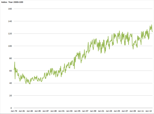
Figure 2: Monthly Truck Tonnage Index, January 1979–December 2013

SOURCE: American Trucking Association, http://www.truckline.com

 

Freight

Domestically, goods are moved by road, air, rail, water, or pipeline as described below. Freight activity is typically measured by tons, value, and ton-miles of cargo moved. Not all metrics are available monthly for all modes.

Trucking (figure 2)

Data on movements by truck are provided through a truck tonnage index, calculated by the American Trucking Associations (ATA); this index is a relative measure of the total tonnage transported by the motor carrier industry for a given month. For the most recent data, BTS uses the preliminary value of the truck tonnage index (provided by ATA); when the official data become available, the preliminary values are replaced.

Air (figure 3)

U.S. air carriers operating between airports located within the boundaries of the United States and its territories report freight ton-miles monthly to BTS. As with the air revenue passenger-miles,⁶ the ton-mile data are drawn from air carrier reports to BTS on Form 41 Schedule T-100, which contains extensive information on air freight movement as well as passenger travel by air.

Rail (figures 4 and 5)

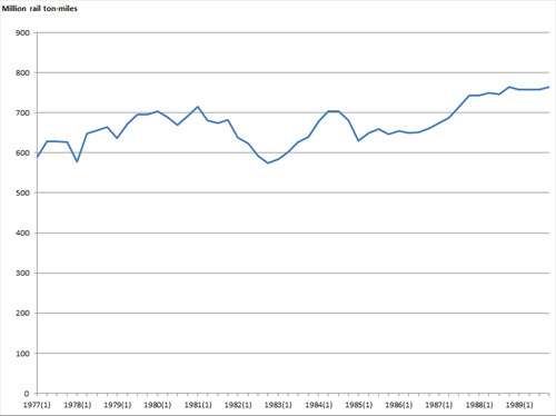
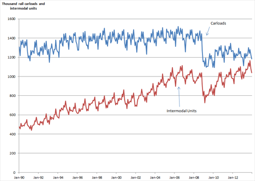
The monthly rail freight data from 1990 to the present (2013) are tabulated from weekly carloads and intermodal units made available by the Association of American Railroads (AAR).⁷ These data are not measured in ton-miles, but their behavior is assumed to be similar to monthly ton-mile totals. For years prior to 1990, these monthly data were not available, so BTS used quarterly rail ton-mile data obtained from the Federal Railroad Administration (FRA). These quarterly values are then expanded, using linear interpolation, to monthly values.⁸

 

Figure 3: Air Revenue Ton-Miles of Freight and Mail, January 1979–December 2013

SOURCE: U. S. Department of Transportation, Bureau of Transportation Statistics, http://www.bts.gov

 

Figure 4: Quarterly Rail Ton-miles, 1st Quarter 1977–4th Quarter 1989

SOURCE: U. S. Department of Transportation, Federal Railroad Administration, http://www.fra.dot.gov

 

Figure 5: Monthly Rail Carloads and Intermodal Units, January 1990–December 2013

SOURCE: Association of American Railroads, http://www.aar.org

 

Water (figure 6)

Waterborne freight includes ton and ton-mile data, collected by the U.S. Army Corp of Engineers (USACE), for internal U.S. waterways. All maritime vessels are required by law to report freight and tonnage to USACE, with the exceptions of the following: military cargo on military vessels; cargo carried on general ferries; fuel products, such as coal and petroleum, loaded from shore facilities directly into vessel bunkers; and insignificant amounts of government materials.

Pipeline (figures 7 and 8)

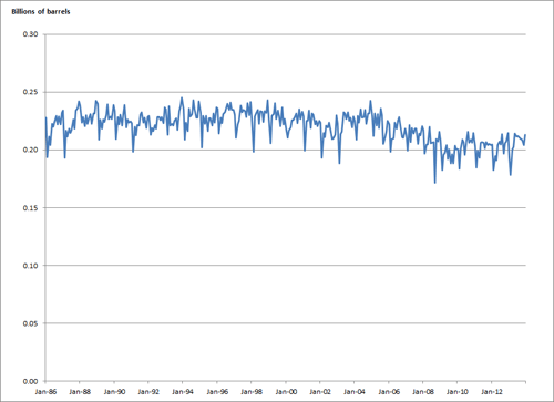
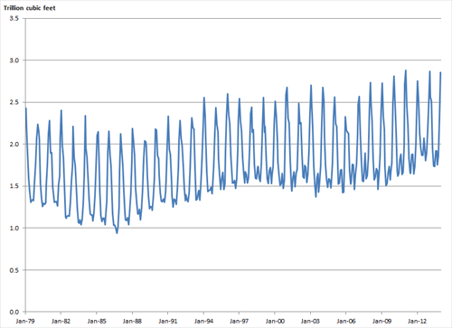
Petroleum supply data and natural gas consumption data are collected by the Office of Energy Statistics in the Energy Information Administration (EIA), U.S. Department of Energy (DOE). The petroleum supply data in the TSI, which consist of the monthly sum of the Alaska petroleum production and the movement between PADDs (Petroleum Administration for Defense Districts), approximate the movement of petroleum.⁹ Natural gas consumption is used as a proxy for the movement of natural gas.

 

Figure 6: Monthly Tonnage Indicator for Internal U.S. Waterways, January 1979–December 2013

SOURCE: U. S. Army Corps of Engineers, Waterborne Commerce Statistics Center, http://www.usace.army.mil

 

Figure 7: Monthly Movement between PADDs by Pipelines plus Alaska Field Production, January 1986–December 2013

SOURCE: U. S. Department of Energy, Energy Information Administration, http://www.eia.gov/dnav/pet/pet_move_pipe_a_ep00_lmv_mbbl_m.htm

 

Figure 8: Monthly Consumption of Natural Gas, January 1979–December 2013

SOURCE: U. S. Department of Energy, Energy Information Administration, http://www.eia.gov/dnav/ng/hist/n9140us2m.htm

 

Passenger

The passenger TSI encompasses three for-hire modes of travel: air, rail, and transit. The passenger TSI does not include movement by personal motor vehicles (including rentals), taxi, and intercity bus services due to the lack of available data.

Air (figure 9)

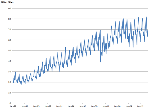
The largest component of the passenger TSI is aviation. Aviation data are collected and compiled from Form 41, Schedule T-100 data submitted to BTS' Office of Airline Information (OAI). The primary source of data, the T-100 dataset, contains extensive information on passenger air travel as well as freight movement by air. The TSI passenger index uses revenue passenger-miles data from the T-100 dataset.

Rail (figure 10)

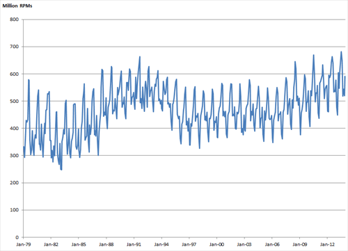
Rail revenue passenger-miles are compiled from the U.S. Department of Transportation, Federal Railroad Administration (FRA) data series for Amtrak and the Alaskan Railroad Corp. Commuter rail is not included in this measure because it is already covered in the transit data.

Transit (figure 11)

The final component of the TSI passenger index is transit. Monthly transit data, primarily from heavy rail and trolleybus agencies as well as nearly all light rail and commuter rail agencies, are collected by the American Public Transportation Association (APTA), and more recently by the Federal Transit Administration. This historical index uses APTA's monthly measure of unlinked trips.¹⁰

 

Figure 9: Monthly Air Revenue Passenger Miles, January 1979–December 2013

SOURCE: U. S. Department of Transportation, Bureau of Transportation Statistics, http://www.bts.gov

 

Figure 10: Monthly Rail Revenue Passenger Miles for AMTRAK and Alaska RR, January 1979–December 2013

SOURCE: U. S. Department of Transportation, Federal Railroad Administration, Office of Safety Analysis, http://www.fra.dot.gov

 

Figure 11: Monthly Unlinked Passenger Trips, January 1979–December 2013

SOURCE: American Public Transportation Association, http://www.apta.com/ resources/statistics/Pages/ridershipreport.aspx

 

Calculation of the TSI

After the data on the individual passenger and freight components have been collected (or estimated), these data series are seasonally adjusted and indexed.¹¹

Seasonal Adjustment, Indexing, Weighting, and Chaining

The previous figures indicate graphically the seasonal nature of the data. In order to portray real growth, X-12-ARIMA was used to deseasonalize the data¹². In applying the X-12 methodology to the transportation services time-series data, BTS noted that each time series component of the TSI displays significant seasonal patterns. (Appendix A provides details on the X-12 ARIMA seasonal adjustment procedure.)

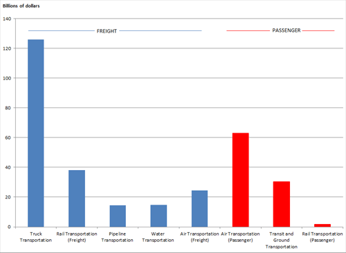
After the individual data series are deseasonalized, the data are indexed using the 12-month average of data from the year 2000 as the base. Each modal series is indexed individually. Then weights for each transportation mode are created using Gross Domestic Product (GDP) valueadded— as reported in the November issue of the Survey of Current Business¹³, issued by the U.S. Department of Commerce's Bureau of Economic Analysis. Inputs to transportation, which are already counted in measures of other sectors, are not included. The index thereby acts as a measure of the economic activity added by the transportation sector itself. Figure 12 provides a graph of the value-added GDP for transportation, represented in billions of dollars for a single year, so the reader can understand the relative impact of the weights.

These annual GDP values undergo several stages of conversion prior to being used as weights. First, the rail and air values are split into passenger and freight values (as shown in figure 12). Next, these monthly values are corrected for double counting by converting to unit value-added GDP. These adjusted value added figures are derived by dividing the modal value-added GDP values by an annual value of the modal quantity index.¹⁴ Finally, annual numbers are linearly interpolated to monthly values.¹⁵

The Fischer Ideal methodology (see Lent, 2004) is used to combine the indexes. Chaining is also used to generate period-to-period changes that are independent of the base year, since period-to-period changes are the focus of the index. When the indexing, weighting, and chaining have been completed, the final three historical indexes are calculated: the total TSI, the passenger TSI, and the freight TSI.

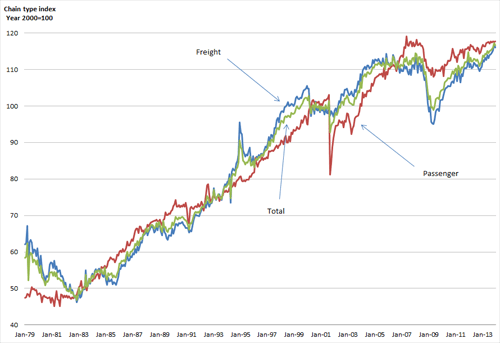
As shown in figure 1, the TSI has experienced upwards growth throughout most of the reference period. Occasional dips and drops are obvious, and the impact of the terrorist attacks of September 11, 2001 is conspicuous. Figure 13 shows the complete history of the TSI, back to 1979. Discussed next is whether the changes in direction of the TSI measures can be related to the changes in direction of the economy.

Business Cycles and the TSI

Transportation services involve the movement of people, goods, and services. All transportation freight services and many transportation passenger services are undertaken to support other economic activities. Freight services move the products produced by the mining, agricultural, and manufacturing sectors of the economy; connect manufacturers to their sources of raw materials, intermediate goods, and spare parts; and provide the goods sold by wholesalers and retailers. Many passenger transportation services are used by business travelers whose travels are directly connected to economic activity. Therefore, one would expect a measure of transportation services to have some relationship to other measures of economic activity, and perhaps track macroeconomic cycles. Indeed, GDP has been identified in the transportation economics literature as one of the key factors whose growth leads to the growth of demand for freight transportation services (Wilson, 1980).

 

Figure 12: Value-Added for TSI Components, 2012

SOURCE: U. S. Department of Transportation, Bureau of Transportation Statistics, http://www.bts.gov

 

Figure 13: Three TSI's: Total, Freight and Passenger, January 1979–December 2013

SOURCE: U. S. Department of Transportation, Bureau of Transportation Statistics, http://www.bts.gov

 

A measure of the output of the transportation sector might be even more valuable if it leads the other economic measures as it could then be used in forecasting those measures as well as macroeconomic cycles. There are a priori reasons to expect transportation to be a precursor of economic activity. Freight transportation activity, for example, is directly tied to the supply chain and to the build-up and maintenance of inventories, and so transportation of finished goods may anticipate growth in sales at the retail and wholesale levels. A very large portion of freight volume consists of raw materials and other intermediate goods, which may be ordered in anticipation of growing activity in the manufacturing sector. Alternatively, a decline in freight shipments may result from anticipations of declines in economic activity in the downstream sectors. The build-up and decline of inventories probably explains why rail traffic figures have historically been used as a general economic indicator (Page and Wirtz, 2003).

Passenger travel could also be a precursor of economic activity. On the one hand, passenger travel, as measured in TSI, is largely a consumer service and could be reasonably inferred to vary with consumer incomes. Being correlated with income should make a measure like this a coincident indicator; i.e., one that varies with changes in the economy, rather than leading them. However, consumer confidence and consumer expectations are widely used as leading economic indicators. It has been suggested by aviation economists¹⁶ that both consumer and business travel may be very sensitive to confidence. Therefore it is possible that a measure of passenger travel is an indicator of confidence (an independent indicator from confidence as measured in surveys), and so passenger travel is a leading indicator. Determining which view of passenger travel is correct, as either a coincident or leading indicator can only be done by examining the evidence, which this paper will do.

These a priori reasons indicate that the transportation sector overall could be strongly related to the general economy. Individual transportation modes have been used in the past as indicators of the business cycle. However, there is reason to expect a multimodal measure of transportation to be superior to any single mode as an indicator of the overall economy, aside from the well-known statistical fact that indexes of several factors are nearly always more stable than single factors. A multimodal measure should be superior as an indicator because, by incorporating all modes, it "absorbs" the competition among the modes and reflects the overall economic change more accurately than a single measure. Railroad carloads, for instance, could decrease if there were a change in the economic situation facing railroad customers and their logistics patterns due to problems in the economy, or the carloads could decrease due to a shift in traffic to waterborne transportation or to trucks. By contrast, an index that incorporates all modes is less subject to such vicissitudes in modal share.

Hence, it is reasonable to expect that changes in a multimodal index are more likely to represent the influence of macroeconomic factors. The TSI freight index works especially well in this regard because "for hire" freight makes up a large portion of all freight movement. While the "for-hire" passenger TSI only includes a small portion of passenger travel because travel by private automobile is excluded, the relationship of passenger travel to the economy could still be strong due to the sizeable component of air travel in the index.

Recessions and Growth Cycles

The majority of cycle research in economics focuses on the business cycle, in which recessions and expansions are identified. In recent years the U.S. economy has experienced fairly long time periods between recessions. Macroeconomists have identified growth cycles that occur within the larger business cycle. Growth cycles represent the cyclical changes in the economy once the long-term trend has been removed. Therefore, growth cycles highlight the accelerations and decelerations in the economy.

If downturns in TSI also signal downturns in the growth cycle, then looking only at these downturns relative to the business cycle while ignoring the growth cycle could cause the TSI to generate "false positives," i.e., indicating a change in the business cycle when no such change followed. This would make TSI an imprecise indicator even if all recessions were preceded by TSI downturns. By calculating growth cycle slowdowns and accelerations¹⁷ for comparison to the TSI, BTS can more completely test the relationship of TSI to the economy. There is no particular reason to expect that the TSI would have a different relationship to growth slowdowns than it would to recessions, both of which would likely impact inventory levels, ordering processes, and other transportation related supply chain factors.

Identification of Turning Points

In 1946 Arthur Burns and Wesley Mitchell wrote the first major paper on business cycle turning points in the American economy. Turning points signal a shift from recession to expansion or expansion to recession, and are found at the trough or the peak of a business cycle. Using hundreds of historic data series, Burns and Mitchell identified clusters of turning points in the overall business cycle. (Burns and Mitchell, 1946)

The fundamental components of the business cycle described by Burns and Mitchell are still used today. However, because it is often not clear which observation is the "true" low or high point of a cycle, methodologies for recognizing turning points have been refined many times during the past 6 decades.

Recession Defined by NBER

The Business Cycle Dating Committee of the National Bureau of Economic Research (NBER) is regarded as the authority on identifying the turning points in business cycles. A recession is often considered a period of two consecutive quarters of decline in Gross Domestic Product (GDP). The Committee defines a recession as "a significant decline in economic activity spread across the economy, lasting more than a few months, normally visible in production, employment, real income, and other indicators."¹⁸ Peaks and troughs are identified by the Committee based on multiple data sources, such as real GDP, real income, employment, industrial production, and wholesale-retail sales.

During the period from 1979 to the present, the Committee found five recessions. However, these shifts in the business cycle were not identified by NBER in real time; each of these recessions was identified several months, or years, after its conclusion. As a result of this time delay, as well its lack of a formal methodology for duplication, the NBER process cannot be used to make real-time declarations about the economic conditions of the country. This delay in recognizing the cyclical turning points exists not only for the business cycle, but for the growth cycles as well, which are discussed next.

Growth Cycles Determined

Economists have noted the existence of growth cycles within a business cycle and these, too, have turning points. Turning points may signal the end points of the expansions and recessions of business cycles, or they may signal the endpoints of growth cycles. A growth cycle is a general slowdown in growth around a trend that continues to grow. As noted by Zarnowitz and Ozyildirim (2001), "growth cycles are generally shorter, more frequent, and much more nearly symmetrical than business cycles." Unlike business cycles, growth cycles are not declared by NBER. Various end points of growth cycles have been identified and are available in academic literature. For this analysis, the TSI team used the approach employed by Zarnowitz and Ozyildirim to identify growth cycles; their research utilized the composite index of coincident economic indicators (CEI), as defined and maintained by the Conference Board, to identify the economy's growth cycles.

Academics have developed procedures that formalize the identification of turning points for business cycles. One technique used as a starting point for many methodologies is an algorithm developed by Bry and Boschan (1971), B&B for short. Application of the B&B algorithm is also the first step in many growth-cycle analyses.¹⁹ Two of the most widely used and academically vetted methodologies, the Phase-Average Trend and the Hodrick-Prescott filter, are used with the B&B technique to detrend the data for more in-depth analysis. The basic procedure for the B&B approach to identifying turning points, summarized in Appendix B²⁰, can be used to measure the turning points in other cycles, e.g., the TSI.

Calculation of TSI Turning Points

TSI and recession cycles

The strong long-terms trends in the time series data cause difficulties in observing changes in possible upturns and downturns of the data. The Hodrick-Prescott (HP) filter is applied to the data in order to detrend the data and observe the underlying cycles more easily.²¹ In its research, BTS chose to use the HP filters with an alpha of 108,000 (as suggested by Zarnowitz and Ozyildirim [2001] and by Lahiri et al. [2003]).

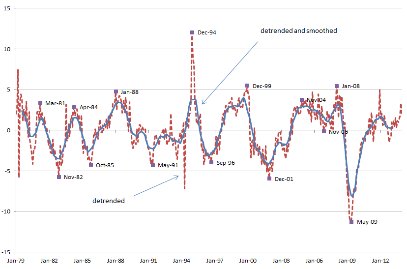
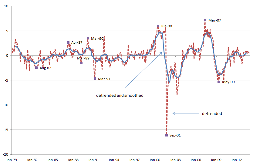
Utilizing the B&B procedure, BTS first took a 12-month centered moving average of the detrended TSI data, then applied the 13-point Spencer curve,²² and finally applied a shorter 3-month moving average to all three series. The 12-month centered moving average allowed identification of the general location of the turns, whereas the Spencer curve and the shorter moving average helped pinpoint the date. Then, by referring back to the original detrended data, BTS selects the peaks and troughs indicated by the moving averages and Spencer curve. To see the resultant peaks and troughs of the two TSI series, figures 14 and 15 illustrate the detrended freight and passenger indexes against their detrended and smoothed counterparts, which are the12-month centered moving averages calculated in the first step in the B&B procedure.

The peaks and troughs in the two indexes were first com - pared to the turning points in the recessions, as identified by the NBER. The detrended TSI results are displayed in table 2, along with the dates of the recessions.

The passenger TSI seems to turn prior to the recessionary peaks and troughs (with one false cycle with a peak in April 1987 and a trough in March 1989), whereas the freight TSI turns more often than the NBER declared recessions. Figure 16 illustrates the accelerations and decelerations of the passenger TSI in relationship to the recessions, shown as shaded areas

The freight TSI seems to lead recessionary peaks more than troughs in the business cycle, suggesting it signals recessions rather than recoveries. This relationship was, however, reversed in the recent recession from December 2007 through June 2009.

The question suggested by table 2 is why the freight index over-signals recessions. We will attempt to validate the relationship between the freight TSI and recessions by next studying the growth cycles.

 

Figure 14: Detrended Freight TSI compared to Detrended and Smoothed Freight TSI January 1979–December 2013

SOURCE: U. S. Department of Transportation, Bureau of Transportation Statistics, http://www.bts.gov

 

Figure 15: Detrended Passenger TSI Compared to Detrended and Smoothed Passenger TSI, January 1979–December 2013

SOURCE: U. S. Department of Transportation, Bureau of Transportation Statistics, http://www.bts.gov

 

Table 2: Dates of Turning Points of Recessions and Detrended Freight and Passenger TSI

	Recessions	Detrended Freight TSI	Detrended Passenger TSI
Peak	Jan-80	N/A	N/A
Trough	Jul-80	N/A	N/A
Peak	Jul-81	Mar-81	N/A
Trough	Nov-82	Nov-82	Aug-82
Peak		Apr-84	Apr-87
Trough		Oct-85	Mar-89
Peak	Jul-90	Jan-88	Mar-90
Trough	Mar-91	May-91	Mar-91
Peak		Dec-94
Trough		Sep-96
Peak	Mar-01	Dec-99	Jun-00
Trough	Nov-01	Dec-01	Sep-01
Peak		Nov-04
Trough		Nov-06
Peak	Dec-07	Jan-08	May-07
Trough	Jun-09	May-09	May-09

NOTE: N/A: Initial start date of the TSI data, and the subsequent smoothing calculations, do not provide enough monthly data to relate to the 1980 recession.

SOURCE: NBER, http://www.nber.org/cycles.html, U.S. Department of Transportation, Bureau of Transportation Statistics, http://www.bts.gov

 

Figure 16: Detrended Passenger TSI, Detrended and Smoothed Passenger TSI, and NBER recessions, January 1979–December 2013

NOTE: Shaded areas indicate U.S recessions, as defined by the National Bureau of Economic Research.

SOURCE: U. S. Department of Transportation, Bureau of Transportation Statistics, http://www.bts.gov

 

TSI and Growth Cycles

As noted in Zarnowitz and Ozyildirim (2001), recession turning points are not the only changes of interest in economic time series: the turning points associated with growth cycles also are of interest. This was first suggested in the original TSOI research performed by Lahiri et al. (2003). The peaks and troughs of the growth cycles were calculated by applying the B&B procedure to the CEI data from the Conference Board. The dates of the peaks and troughs of the TSI data were then compared against the turns in the growth cycles, as shown in table 3.

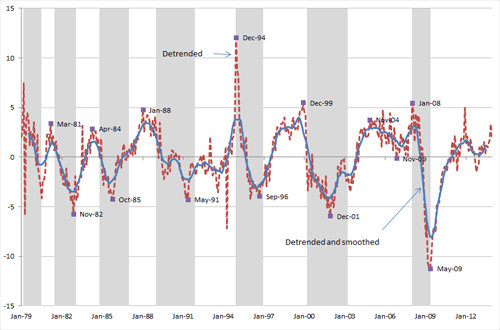
The freight TSI tends to lead the identified growth cycles at the peaks as well as at the troughs. Only one false cycle occurred in the freight TSI– with a peak in November 2004 and a trough in November 2006. Figure 17 illustrates the relationship between the freight TSI and growth cycles, shown as shaded areas.

Conclusions and Future Research

The historical passenger TSI anticipated the four recent NBER declared recessions since 1981, but experienced an additional cycle that was not related to a recession. The historical freight TSI anticipated the four NBER declared recessions in this time period, but there were other turns in the index that did not precede declared recessions or expansions. The final comparison of the turning points in the freight TSI against the turning points in the growth cycles, however, indicated a strong relationship, with only one additional cycle not related to a growth cycle.

As discussed in the section, Business Cycles and the TSI, there is a priori reason to expect both the freight TSI and the passenger TSI to have relationships to economic cycles. It is not surprising that freight transport could lead business cycles and growth cycles based on the literature and the ties between freight and the general economy. With theory supported by our empirical findings, BTS can expect the leading characteristic of the freight TSI to continue in the future.

As also discussed, there are a priori arguments that the passenger TSI could either lead or be coincident with changes in the broader economy. The empirical data thus far suggests the passenger TSI does in fact lead the business cycle. This means the passenger TSI, as well as the freight TSI, moves in anticipation of broader changes in the economy. The passenger TSI, however, leads turning points in the business cycle, rather than the economic growth cycle. The freight TSI turns down before slowdowns in economic growth, which sometimes do not coincide with recessions, and when they do tend to come earlier than recessions. However the passenger TSI turns down only before actual recessions themselves. This may be because the passenger TSI is driven more by sectors in the economy which, while they turn negative before a recession begins, are less sensitive to a slowdown in growth than the sectors that impact freight transportation. While the reason for this difference between the passenger TSI and the freight TSI should be explored in future research, the empirical result is that both play a role in understanding cyclical changes in the economy. In addition, research should and will be conducted to compare the TSI to other indexes used as leading indicators. The degrees of lead for both TSI are provided in tables 4 and 5.

 

Table 3: Dates of Turning Points of Growth Cycles and Detrended Freight and Passenger TSI

	Growth Cycles	Detrended Freight TSI	Detrended Passenger TSI
Peak	Mar-79	N/A	N/A
Trough	Jul-80	N/A	N/A
Peak	Jul-81	Mar-81	N/A
Trough	Feb-83	Nov-82	Aug-82
Peak	Nov-84	Apr-84	Apr-87
Trough	Jan-87	Oct-85	Mar-89
Peak	Jan-89	Jan-88	Mar-90
Trough	Dec-91	May-91	Mar-91
Peak	Dec-94	Dec-94
Trough	Jan-97	Sep-96
Peak	Apr-00	Dec-99	Jun-00
Trough	Apr-03	Dec-01	Sep-01
Peak		Nov-04
Trough		Nov-06
Peak	Jan-08	Jan-08	May-07
Trough	Jun-09	May-09	May-09

KEY: N/A=not available; initial start date of the TSI data, and the subsequent smoothing calculations, do not provide enough monthly data to relate to the 1979–1980 growth cycle.

SOURCE: NBER, http://www.nber.org/cycles.html, U.S. Department of Transportation, Bureau of Transportation Statistics, http://www.bts.gov

 

Figure 17: Detrended Freight TSI, Detrended and Smoothed Freight TSI and Growth Cycles, January 1979–December 2013

NOTE: Shaded areas indicate growth cycles.

SOURCE: U. S. Department of Transportation, Bureau of Transportation Statistics, http://www.bts.gov

 

It may be difficult to use this information in real-time to predict changes in the economy through the turns in the TSI. Because the employed procedures utilize moving averages, six months of the most recent data are lost in the analysis. By BTS calculations, the TSI leads by less than that amount, thereby making it difficult to use the index as a predictor in real-time. In addition, several months of data after the turning point are needed to ascertain if the change in direction is more than just due to local variation. This additional requirement for monthly data further limits the ability to use the TSI as a real-time predictor of turning points in the economy, but it does not weaken the findings in the historical data. Transportation services appear to lead the economy.

 

Table 4: Recessions and Passenger TSI: Degree of Lead

	Economy	Passenger TSI	Lead (+) / Lag (-)
Peak	Jul-81
Trough	Nov-82	Aug-82	+3
Peak		Apr-87	NA
Trough		Mar-89	NA
Peak	Jul-90	Mar-90	+4
Trough	Mar-91	Mar-91	0
Peak	Mar-01	Jun-00	+9
Trough	Nov-01	Sep-01	+2
Peak	Dec-07	May-07	+7
Trough	Jun-09	May-09	+1

SOURCE: U. S. Department of Transportation, Bureau of Transportation Statistics, http://www.bts.gov

 

Table 5: Growth Cycles and Freight TSI: Degree of Lead

	Economy	Passenger TSI	Lead (+) / Lag (-)
Peak	Jul-81
Trough	Nov-82	Aug-82	+3
Peak		Apr-87	NA
Trough		Mar-89	NA
Peak	Jul-90	Mar-90	+4
Trough	Mar-91	Mar-91	0
Peak	Mar-01	Jun-00	+9
Trough	Nov-01	Sep-01	+2
Peak	Dec-07	May-07	+7
Trough	Jun-09	May-09	+1

SOURCE: U. S. Department of Transportation, Bureau of Transportation Statistics, http://www.bts.gov

 

For more information, contact:

Ken Notis, Economist
Bureau of Transportation Statistics
U.S Department of Transportation
1200 New Jersey Ave., SE (Room E34-436)
Washington, DC 20590
Email: ken.notis@dot.gov
Phone: 202-366-3576

References

Burns A. and W. Mitchell. 1946. Measuring Business Cycles. New York, NY: National Bureau of Economic Research.

Bry, G. and C. Boshan. 1971. Cyclical Analysis of Time Series: Selected Procedures and Computer Programs, NBER Technical Paper 20. Cambridge, MA: National Bureau of Economic Research.

Cashin, Paul, and Sam Ouliaris. "Key Features of Australian Business Cycles." Australian Economic Papers 43.1 (2004): 39-58.

Harding, Don, and Adrian Pagan. Measurement of Business Cycles. No. 966. 2006.

Hodrick, R. and E. Prescott. 1997. Postwar U.S. Business Cycles: An Empirical Investigation. Journal of Money, Credit and Banking, 29(1), 1-16.

Kendall, M. and K. Ord. 1990. Time Series, 3rd ed. London, UK: Edward Arnold.

King, Robert G., and Charles I. Plosser. "Real Business Cycles and the Test of the Adelmans." Journal of Monetary Economics 33.2 (1994): 405-438.

Lahiri, K and H. Stekler. 2002. The Theoretical Development, Selection, and Testing of Economic Indicators for the Transportation Industry, BTS Research Grant Final Report. Washington, DC: Bureau of Transportation Statistics.

Lahiri, K., H. Stekler, W. Yao and P. Young. 2003. Monthly Output for the U.S. Transportation Sector. Journal of Transportation and Statistics 6(2/3), 1-28.

Lahiri, K., W. Yao and P. Young. 2004. Transportation and the Economy: Linkages at Business-Cycle Frequencies. Transportation Research Record: Journal of the Transportation Research Board, No. 1864, 103-111.

Ladiray, D. and B. Quenneville. 2001. Seasonal Adjustment with X-11 Method. New York, NY: Springer.

Lent, J. 2004. Effects of Extreme Values in Price Indexes: The Case of the Air Travel Price Index. Journal of Transportation and Statistics 7(2/3), 41-52.

Page, D. and R. Wirtz. 2003. Wrong Side of the Tracks. Fedgazette, Federal Reserve Bank of Minneapolis, November 2003.

Wilson, G. 1980. Economic Analysis of Intercity Freight Transportation. Bloomington, Indiana: Indiana University Press.

Zarnowitz, V. and A. Ozyildirim. 2001. Time Series Decomposition and Measurement of Business Cycles, Trends and Growth Cycles, Economics Program Working Paper #01-04. New York, NY: The Conference Board.

Appendix A: Details on Seasonal Adjustment

The data used for the Transportation Services Index are seasonally adjusted by a method that evolved over many decades starting in the 1950s at the U.S. Bureau of Census. Called X-12-ARIMA, Release 0.2, this procedure recently evolved out of the "X-11 Variant of the Census Method II Seasonal Adjustment Program." The name, X-11, means 11 variations precede it.

Fundamentally, X-12 (without ARIMA) is a robust non-parametric method, which achieves its estimates through a series of iterative steps. As such, it is an "empirical" approach as distinguished from a "model-based" approach to seasonal adjustment. This means that the statistical properties of the estimators, such as confidence intervals, are lacking for the adjusted series. This is not highly concerning as the seasonal adjustments of the transportation series used in the TSI are relatively small.

ARIMA modeling was added to X-11 methods in 1975, thereby providing a popular statistical component to an iterative approach of successive smoothings. The ARIMA was introduced to model the data to produce forecasts that are used to extend the data series before undergoing the adjustments and smoothings. The seasonal adjustments were then found to be more reliable as measured by the reductions in revisions of estimates near the end of the series.

ARIMA modeling is part of the X-12 package used to seasonally adjust the TSI data series. Table A-1 summarizes the characteristics of the model used.

 

Table A-1

Models for seasonal adjustment of TSI data inputs

Mode	Model1	Trading days2 and holidays3	Outliers4	ARIMA
Rail
Passenger	A	TD; Easter[7], Labor Day, Thanksgiving_7	None	(0,1,1)(0,1,1)
Rail Freight
Carloads	A	No TD; Leap year	LS DEC2008	(0,1,1)(0,1,1)
Intermodals	M	No TD; Leap year; Easter[7], Memorial Day, Thanksgiving_8, Christmas	AO OCT2002; LS DEC2008	(0,1,1)(0,1,1)
Trucking	A	TD_1; No holidays	LS MAR2000	(2,1,1)(0,1,1)
Waterborne	A	No TD; No holidays	AO JAN2000; AO MAY2011	(0,1,2)(0,1,1)
Transit	A	TD; No holidays	AO MAY2007	(0,1,1)(0,1,1)
Aviation
Freight	M	TD_1; Easter[2], Memorial Day, Thanksgiving_8	AO SEP2001; TC OCT2002; LS NOV2008;	(0,1,2)(0,1,1)
Passenger	A	No TD; Easter, Thanksgiving_8	AO SEP2001; LS OCT2001	(0,1,1)(0,1,1)
Pipeline
Natural gas	M	No TD; Leap year; No holidays	None	(0,1,2)(0,1,1)
Petroleum	A	No TD; Leap year; No holidays	AO SEP2008	(0,1,2)(0,1,1)

¹ M = Multiplicative; A = Additive

² TD = Trading Days Monday through Saturday versus Sunday; TD_1 = Weekday versus Weekend

³ Moving Holidays/Calendar Effects = Easter, Memorial Day, Labor Day, Thanksgiving, and Christmas.

Easter[n] = number of days n before Easter

Easter = Thursday before to Tuesday after (6 days).

Memorial Day = Friday before to the Tuesday after (5 days).

Labor Day = Friday before to Tuesday after (5 days).

Thanksgiving_7 = Tuesday before to Sunday after (7 days)

Thanksgiving_8 = Tuesday before to Monday after (8 days).

Christmas

If Christmas falls on a Monday = Friday before through Tuesday after (12 days).

If Christmas falls on a Friday = Wednesday through Sunday after (12 days).

If Christmas falls on a Saturday = Wednesday through Sunday after (12 days).

If Christmas falls on a Sunday = Thursday through Monday after (12 days).

⁴ LS = Level Shift; AO = Automatic Outlier; TC = Temporary Change

 

Appendix B: Bry and Boschan Procedure

• Determination of extremes and substitution of values.
• Determination of cycles in 12-month moving average (extremes replaced).
  • Identification of points higher (or lower) than 5 months on either side.
  • Enforcement of alternation of turns by selecting highest of multiple peaks (or lowest of multiple troughs).
• Determination of corresponding turns in Spencer Curve (extremes replaced).
  • Identification of highest (or lowest) value within ± 5 months of selected turn in 12-month moving average.
  • Enforcement of minimum cycle duration of 15 months by eliminating lower peaks and higher troughs of shorter cycles.
• Determination of corresponding turns in short-term moving average of 3 to 6 months, depending on MCD (months of cyclical dominance).
  • Identification of highest (or lowest) value within ± 5 months of selected turn in Spencer curve.
• Determination of turning points in unsmoothed series.
  • Identification of highest (or lowest) value within ± 4 months of selected turn in short-term moving average.
  • Elimination of turns within 6 months of beginning and end of series.
  • Elimination of peaks (or troughs) at both ends of series which are lower (or higher) than values closer to end.
  • Elimination of cycles whose duration is less than 15 months.
  • Elimination of phases whose duration is less than 5 months.
• Statement of final turning points.

 

¹ For this report, the analyses are conducted through December 2013.

² The National Bureau of Economic Research (NBER) declared recessions from January 1980 – July 1980, July 1981—November 1982, July 1990 – March 1991, March 2001 – November 2001, and December 2007 – June 2009.

³ Highway, air, railway, waterway, and pipeline.

⁴http://www.rita.dot.gov/bts/sites/rita.dot.gov.bts/files/Transportation%...

⁵ For further detail regarding the data sources, the reader can refer to the TSI webpage on the BTS website: http://www.bts.gov/programs/economics_and_finance/ transportation_services_index/html/source_and_documentation_and_data_quality.html

⁶ A passenger-mile equals 1 passenger transported 1 mile. For example, 75 passengers transported 1,000 miles would equal 75,000 passenger-miles.

⁷ The AAR data can be obtained from the Weekly Railfax Rail Carloading Report, from Atlantic Systems Inc., http://railfax.transmatch.com

⁸ SAS is employed to perform the linear interpolation, through the JOIN method in Proc EXPAND. The JOIN method fits a continuous curve to the data by connecting successive straight line segments.

⁹ The petroleum pipeline data are only available back to 1986. This means that for 1979 through 1985, the freight component of the index does NOT include pipeline data. Rather, the pipeline data are spliced into the freight TSI, starting in 1986.

¹⁰ The number of passengers who board public transportation vehicles. Passengers are counted each time they board vehicles no matter how many vehicles they use to travel from their origin to their destination.

¹¹ For additional detail, see Technical Note: DOCUMENTATION for the Transportation Services Index at: http://www.rita.dot.gov/bts/sites/rita.dot.gov.bts/files/subject_areas/ economics_and_finance/transportation_services_index/documentation/index.html

¹² For an excellent reference on X-12-ARIMA, see Ladiray and Quenneville (2001)

¹³https://bea.gov/scb/date_guide.asp

¹⁴ The reason to create these 'adjusted' value-added figures, rather than valueadded, as the proxy for "price" is because the unit value added allows the TSI to get rid of the "double counting" effect of the changes in output level that is embodied in the value-added of the industry.

¹⁵ Details on the changes in the weights can be found in the TSI documentation: http://www.rita.dot.gov/bts/sites/rita.dot.gov.bts/files/subject_areas/e... finance/transportation_services_index/documentation/index.html

¹⁶ Personal conversations with Federal Aviation Administration, January 2014.

¹⁷ See Zarnowitz and Ozyildirim (2001) for a study of growth cycles as related to business cycles.

¹⁸http://www.nber.org/cycles/dec2008.html

¹⁹ Examples of the B&B algorithm can be found in Harding and Pagan (2006), King and Plosser (1994), and Cashin and Ouliaris (2004), to name a few.

²⁰ Taken from Bry and Boschan (1971), Table I, page 21.

²¹ See Hodrick and Prescott (1997) for more detail.

²² The Spencer curve is a smoothing formula that uses simple averages to approximate more complex quadratic equations. For further information, see Kendall and Ord (1990).