

§3.6 Linear Difference Equations
- Keywords:
- difference equations
- Referenced by:
- §11.13(v), §14.32, §18.40, §28.34(iii), §29.20(i), Ch.3, §30.16(ii), §33.23(iv)
- Permalink:
- http://dlmf.nist.gov/3.6
Contents
- §3.6(i) Introduction
- §3.6(ii) Homogeneous Equations
- §3.6(iii) Miller’s Algorithm
- §3.6(iv) Inhomogeneous Equations
- §3.6(v) Olver’s Algorithm
- §3.6(vi) Examples
- §3.6(vii) Linear Difference Equations of Other Orders
§3.6(i) Introduction
- Defines:
 : forward difference operator
- Referenced by:
- §2.9(i), §26.8(v)
- Permalink:
- http://dlmf.nist.gov/3.6.i
Many special functions satisfy second-order recurrence relations, or difference equations, of the form
- Symbols:
-
 : sequence,
  : coefficient,
  : coefficient,
  : coefficient and
  : coefficient
- Referenced by:
- §3.6(iv), §3.6(v)
- Permalink:
- http://dlmf.nist.gov/3.6.E1
- Encodings:
- TeX, pMML, png
or equivalently,
- Symbols:
-
: forward difference operator, : sequence, : coefficient, : coefficient, : coefficient and : coefficient
- Permalink:
- http://dlmf.nist.gov/3.6.E2
- Encodings:
- TeX, pMML, png
where ![]() ,
,
![]() , and
, and ![]() . If
. If
![]() ,
, ![]() , then the difference equation is homogeneous;
otherwise it is inhomogeneous.
, then the difference equation is homogeneous;
otherwise it is inhomogeneous.
§3.6(ii) Homogeneous Equations
- Keywords:
- backward recursion, difference equations
- Referenced by:
- §15.19(iv), §3.6(i)
- Permalink:
- http://dlmf.nist.gov/3.6.ii
Given numerical values of ![]() and
and ![]() , the solution
, the solution ![]() of the equation
of the equation
- Symbols:
-
: sequence, : coefficient, : coefficient and : coefficient
- Referenced by:
- §3.6(ii), §3.6(ii), §3.6(v), §3.6(v)
- Permalink:
- http://dlmf.nist.gov/3.6.E3
- Encodings:
- TeX, pMML, png
with ![]() ,
, ![]() , can be computed recursively for
, can be computed recursively for
![]() . Unless exact arithmetic is being used, however, each step of
the calculation introduces rounding errors. These errors have the effect of
perturbing the solution by unwanted small multiples of
. Unless exact arithmetic is being used, however, each step of
the calculation introduces rounding errors. These errors have the effect of
perturbing the solution by unwanted small multiples of ![]() and of an
independent solution
and of an
independent solution ![]() , say. This is of little consequence if the wanted
solution is growing in magnitude at least as fast as any other solution of
(3.6.3), and the recursion process is stable.
, say. This is of little consequence if the wanted
solution is growing in magnitude at least as fast as any other solution of
(3.6.3), and the recursion process is stable.
But suppose that ![]() is a nontrivial solution such that
is a nontrivial solution such that
Then ![]() is said to be a recessive (equivalently, minimal or
distinguished) solution as
is said to be a recessive (equivalently, minimal or
distinguished) solution as ![]() , and it is unique
except for a constant factor. In this situation the unwanted multiples of
, and it is unique
except for a constant factor. In this situation the unwanted multiples of ![]() grow more rapidly than the wanted solution, and the computations are
unstable. Stability can be restored, however, by backward
recursion, provided that
grow more rapidly than the wanted solution, and the computations are
unstable. Stability can be restored, however, by backward
recursion, provided that ![]() ,
, ![]() : starting from
: starting from ![]() and
and
![]() , with
, with ![]() large, equation (3.6.3) is applied to generate
in succession
large, equation (3.6.3) is applied to generate
in succession ![]() . The unwanted multiples of
. The unwanted multiples of ![]() now decay in comparison with
now decay in comparison with ![]() , hence are of little consequence.
, hence are of little consequence.
§3.6(iii) Miller’s Algorithm
- Keywords:
- Miller’s algorithm, difference equations
- Referenced by:
- ¶ ‣ §3.6(vi), §3.6(ii), §6.18(ii)
- Permalink:
- http://dlmf.nist.gov/3.6.iii
Because the recessive solution of a homogeneous equation is the fastest growing
solution in the backward direction, it occurred to J.C.P. Miller
(Bickley et al. (1952, pp. xvi–xvii)) that arbitrary “trial values” can be
assigned to ![]() and
and ![]() , for example, 1 and 0. A “trial solution”
is then computed by backward recursion, in the course of which the original
components of the unwanted solution
, for example, 1 and 0. A “trial solution”
is then computed by backward recursion, in the course of which the original
components of the unwanted solution ![]() die away. It therefore remains to
apply a normalizing factor
die away. It therefore remains to
apply a normalizing factor ![]() . The process is then repeated with a
higher value of
. The process is then repeated with a
higher value of ![]() , and the normalized solutions compared. If agreement is not
within a prescribed tolerance the cycle is continued.
, and the normalized solutions compared. If agreement is not
within a prescribed tolerance the cycle is continued.
The normalizing factor ![]() can be the true value of
can be the true value of ![]() divided by its
trial value, or
divided by its
trial value, or ![]() can be chosen to satisfy a known property of the
wanted solution of the form
can be chosen to satisfy a known property of the
wanted solution of the form

- Symbols:
-
: sequence and
 : constants
- Permalink:
- http://dlmf.nist.gov/3.6.E5
- Encodings:
- TeX, pMML, png
where the ![]() ’s are constants. The latter method is usually superior when the
true value of
’s are constants. The latter method is usually superior when the
true value of ![]() is zero or pathologically small.
is zero or pathologically small.
For further information on Miller’s algorithm, including examples, convergence proofs, and error analyses, see Wimp (1984, Chapter 4), Gautschi (1967, 1997b), and Olver (1964a). See also Gautschi (1967) and Gil et al. (2007a, Chapter 4) for the computation of recessive solutions via continued fractions.
§3.6(iv) Inhomogeneous Equations
- Notes:
- See Olver (1967a).
- Keywords:
- boundary-value methods or problems, difference equations
- Referenced by:
- §3.6(v)
- Permalink:
- http://dlmf.nist.gov/3.6.iv
Similar principles apply to equation (3.6.1) when ![]() ,
,
![]() , and
, and ![]() for some, or all, values of
for some, or all, values of ![]() . If, as
. If, as
![]() , the wanted solution
, the wanted solution ![]() grows (decays) in magnitude at least
as fast as any solution of the corresponding homogeneous equation, then forward
(backward) recursion is stable.
grows (decays) in magnitude at least
as fast as any solution of the corresponding homogeneous equation, then forward
(backward) recursion is stable.
A new problem arises, however, if, as ![]() , the asymptotic behavior
of
, the asymptotic behavior
of ![]() is intermediate to those of two independent solutions
is intermediate to those of two independent solutions ![]() and
and ![]() of the corresponding inhomogeneous equation (the complementary functions). More
precisely, assume that
of the corresponding inhomogeneous equation (the complementary functions). More
precisely, assume that ![]() ,
, ![]() for all sufficiently large
for all sufficiently large
![]() , and as
, and as ![]()
- Symbols:
-
: sequence and
 : solution
- Permalink:
- http://dlmf.nist.gov/3.6.E6
- Encodings:
- TeX, TeX, pMML, pMML, png, png
Then computation of ![]() by forward recursion is unstable. If it also happens
that
by forward recursion is unstable. If it also happens
that ![]() as
as ![]() , then computation of
, then computation of ![]() by backward
recursion is unstable as well. However,
by backward
recursion is unstable as well. However, ![]() can be computed successfully in
these circumstances by boundary-value methods, as follows.
can be computed successfully in
these circumstances by boundary-value methods, as follows.
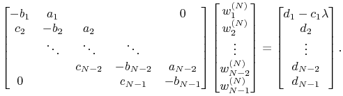
Let us assume the normalizing condition is of the form ![]() , where
, where
![]() is a constant, and then solve the following tridiagonal system of
algebraic equations for the unknowns
is a constant, and then solve the following tridiagonal system of
algebraic equations for the unknowns
![]() ; see §3.2(ii).
Here
; see §3.2(ii).
Here ![]() is an arbitrary positive integer.
is an arbitrary positive integer.
- Symbols:
-
: sequence,
 : arbitrary positive integer, : coefficient, : coefficient, : coefficient, : coefficient and
  : constant
- Permalink:
- http://dlmf.nist.gov/3.6.E7
- Encodings:
- TeX, pMML, png
Then as ![]() with
with ![]() fixed,
fixed, ![]() .
.
§3.6(v) Olver’s Algorithm
- Keywords:
- Olver’s algorithm, difference equations
- Referenced by:
- §10.74(iv), §13.29(iv), ¶ ‣ §3.6(vi), ¶ ‣ §3.6(vi), §3.6(ii), §3.7(iii)
- Permalink:
- http://dlmf.nist.gov/3.6.v
To apply the method just described a succession of values can be prescribed for
the arbitrary integer ![]() and the results compared. However, a more powerful
procedure combines the solution of the algebraic equations with the
determination of the optimum value of
and the results compared. However, a more powerful
procedure combines the solution of the algebraic equations with the
determination of the optimum value of ![]() . It is applicable equally to the
computation of the recessive solution of the homogeneous equation
(3.6.3) or the computation of any solution
. It is applicable equally to the
computation of the recessive solution of the homogeneous equation
(3.6.3) or the computation of any solution ![]() of the
inhomogeneous equation (3.6.1) for which the conditions of
§3.6(iv) are satisfied.
of the
inhomogeneous equation (3.6.1) for which the conditions of
§3.6(iv) are satisfied.
Suppose again that ![]() ,
, ![]() is given, and we wish to calculate
is given, and we wish to calculate
![]() to a prescribed relative accuracy
to a prescribed relative accuracy ![]() for a given
value of
for a given
value of ![]() . We first compute, by forward recurrence, the solution
. We first compute, by forward recurrence, the solution ![]() of
the homogeneous equation (3.6.3) with initial values
of
the homogeneous equation (3.6.3) with initial values ![]() ,
,
![]() . At the same time we construct a sequence
. At the same time we construct a sequence ![]() ,
, ![]() ,
defined by
,
defined by
- Symbols:
-
 : solutions,
  : sequence, : coefficient, : coefficient and : coefficient
- Permalink:
- http://dlmf.nist.gov/3.6.E8
- Encodings:
- TeX, pMML, png
beginning with ![]() . (This part of the process is equivalent to forward
elimination.) The computation is continued until a value
. (This part of the process is equivalent to forward
elimination.) The computation is continued until a value ![]() (
(![]() ) is
reached for which
) is
reached for which
- Symbols:
-
: arbitrary positive integer,
 : relative accuracy,
  : order, : solutions and : sequence
- Referenced by:
- ¶ ‣ §3.6(vi)
- Permalink:
- http://dlmf.nist.gov/3.6.E9
- Encodings:
- TeX, pMML, png
Then ![]() is generated by backward recursion from
is generated by backward recursion from
- Symbols:
-
: sequence, : solutions and : sequence
- Permalink:
- http://dlmf.nist.gov/3.6.E10
- Encodings:
- TeX, pMML, png
starting with ![]() . (This part of the process is back substitution.)
. (This part of the process is back substitution.)
§3.6(vi) Examples
¶ Example 1. Bessel Functions
The difference equation
is satisfied by ![]() and
and ![]() , where
, where
![]() and
and ![]() are the Bessel functions of the first
kind. For large
are the Bessel functions of the first
kind. For large ![]() ,
,
- Symbols:
-
 : Bessel function of the first kind,
  : base of exponential function and
  : asymptotic equality
- Permalink:
- http://dlmf.nist.gov/3.6.E12
- Encodings:
- TeX, pMML, png

- Symbols:
-
 : Bessel function of the second kind, : base of exponential function and : asymptotic equality
- Permalink:
- http://dlmf.nist.gov/3.6.E13
- Encodings:
- TeX, pMML, png
(§10.19(i)). Thus ![]() is dominant and can be computed
by forward recursion, whereas
is dominant and can be computed
by forward recursion, whereas ![]() is recessive and has to be
computed by backward recursion. The backward recursion can be carried out using
independently computed values of
is recessive and has to be
computed by backward recursion. The backward recursion can be carried out using
independently computed values of ![]() and
and ![]() or
by use of Miller’s algorithm (§3.6(iii)) or Olver’s algorithm
(§3.6(v)).
or
by use of Miller’s algorithm (§3.6(iii)) or Olver’s algorithm
(§3.6(v)).
¶ Example 2. Weber Function
The Weber function ![]() satisfies
satisfies
for ![]() , and as
, and as ![]()
- Symbols:
-
 : Weber function and : asymptotic equality
- Permalink:
- http://dlmf.nist.gov/3.6.E15
- Encodings:
- TeX, pMML, png
- Symbols:
-
: Weber function and : asymptotic equality
- Permalink:
- http://dlmf.nist.gov/3.6.E16
- Encodings:
- TeX, pMML, png
see §11.11(ii). Thus the asymptotic behavior of the particular
solution ![]() is intermediate to those of the complementary
functions
is intermediate to those of the complementary
functions ![]() and
and ![]() ; moreover, the conditions for
Olver’s algorithm are satisfied. We apply the algorithm to compute
; moreover, the conditions for
Olver’s algorithm are satisfied. We apply the algorithm to compute
![]() to 8S for the range
to 8S for the range ![]() , beginning with the
value
, beginning with the
value ![]() obtained from the Maclaurin series
expansion (§11.10(iii)).
obtained from the Maclaurin series
expansion (§11.10(iii)).
In the notation of §3.6(v) we have ![]() and
and
![]() . The least value of
. The least value of ![]() that satisfies
(3.6.9) is found to be 16. The results of the computations are
displayed in Table 3.6.1. The values of
that satisfies
(3.6.9) is found to be 16. The results of the computations are
displayed in Table 3.6.1. The values of ![]() for
for
![]() are the wanted values of
are the wanted values of ![]() . (It should
be observed that for
. (It should
be observed that for ![]() ,
however, the
,
however, the ![]() are progressively poorer approximations to
are progressively poorer approximations to ![]() :
the underlined digits are in error.)
:
the underlined digits are in error.)
| 0 | 0.00000 000 | −0.56865 663 | −0.56865 663 | |||||
| 1 | 0.10000 000 | ×10¹ | 0.70458 291 | 0.35229 146 | 0.43816 243 | |||
| 2 | 0.20000 000 | ×10¹ | 0.70458 291 | 0.50327 351 | ×10⁻¹ | 0.17174 195 | ||
| 3 | 0.70000 000 | ×10¹ | 0.96172 597 | ×10¹ | 0.34347 356 | ×10⁻¹ | 0.24880 538 | |
| 4 | 0.40000 000 | ×10² | 0.96172 597 | ×10¹ | 0.76815 174 | ×10⁻³ | 0.47850 795 | ×10⁻¹ |
| 5 | 0.31300 000 | ×10³ | 0.40814 124 | ×10³ | 0.42199 534 | ×10⁻³ | 0.13400 098 | |
| 6 | 0.30900 000 | ×10⁴ | 0.40814 124 | ×10³ | 0.35924 754 | ×10⁻⁵ | 0.18919 443 | ×10⁻¹ |
| 7 | 0.36767 000 | ×10⁵ | 0.47221 340 | ×10⁵ | 0.25102 029 | ×10⁻⁵ | 0.93032 343 | ×10⁻¹ |
| 8 | 0.51164 800 | ×10⁶ | 0.47221 340 | ×10⁵ | 0.11324 804 | ×10⁻⁷ | 0.10293 811 | ×10⁻¹ |
| 9 | 0.81496 010 | ×10⁷ | 0.10423 616 | ×10⁸ | 0.87496 485 | ×10⁻⁸ | 0.71668 638 | ×10⁻¹ |
| 10 | 0.14618 117 | ×10⁹ | 0.10423 616 | ×10⁸ | 0.24457 824 | ×10⁻¹⁰ | 0.65021 292 | ×10⁻² |
| 11 | 0.29154 738 | ×10¹⁰ | 0.37225 201 | ×10¹⁰ | 0.19952 026 | ×10⁻¹⁰ | 0.58373 946 | ×10⁻¹ |
| 12 | 0.63994 242 | ×10¹¹ | 0.37225 201 | ×10¹⁰ | 0.37946 279 | ×10⁻¹³ | ×10⁻² | |
| 13 | 0.15329 463 | ×10¹³ | 0.19555 304 | ×10¹³ | 0.32057 909 | ×10⁻¹³ | ×10⁻¹ | |
| 14 | 0.39792 611 | ×10¹⁴ | 0.19555 304 | ×10¹³ | 0.44167 174 | ×10⁻¹⁶ | ×10⁻² | |
| 15 | 0.11126 602 | ×10¹⁶ | 0.14186 384 | ×10¹⁶ | 0.38242 250 | ×10⁻¹⁶ | ×10⁻¹ | |
| 16 | 0.33340 012 | ×10¹⁷ | 0.14186 384 | ×10¹⁶ | 0.39924 861 | ×10⁻¹⁹ | ||
- Symbols:
-
: Weber function, : sequence, : solutions and : sequence
- Keywords:
- Olver’s algorithm, difference equations
- Referenced by:
- ¶ ‣ §3.6(vi)
- Permalink:
- http://dlmf.nist.gov/3.6.T1
§3.6(vii) Linear Difference Equations of Other Orders
- Keywords:
- boundary-value methods or problems, difference equations
- Referenced by:
- §16.25, §3.6(i)
- Permalink:
- http://dlmf.nist.gov/3.6.vii
Similar considerations apply to the first-order equation
- Symbols:
-
: sequence, : coefficient, : coefficient and : coefficient
- Permalink:
- http://dlmf.nist.gov/3.6.E17
- Encodings:
- TeX, pMML, png
Thus in the inhomogeneous case it may sometimes be necessary to recur backwards to achieve stability. For analyses and examples see Gautschi (1997b).
For a difference equation of order ![]() (
(![]() ),
),
- Symbols:
-
: sequence, : coefficient and : coefficient
- Permalink:
- http://dlmf.nist.gov/3.6.E18
- Encodings:
- TeX, pMML, png
or for systems of ![]() first-order inhomogeneous equations, boundary-value
methods are the rule rather than the exception. Typically
first-order inhomogeneous equations, boundary-value
methods are the rule rather than the exception. Typically ![]() conditions
are prescribed at the beginning of the range, and
conditions
are prescribed at the beginning of the range, and ![]() conditions at the end.
Here
conditions at the end.
Here ![]() , and its actual value depends on the asymptotic behavior
of the wanted solution in relation to those of the other solutions. Within this
framework forward and backward recursion may be regarded as the special cases
, and its actual value depends on the asymptotic behavior
of the wanted solution in relation to those of the other solutions. Within this
framework forward and backward recursion may be regarded as the special cases
![]() and
and ![]() , respectively.
, respectively.