

§3.1 Arithmetics and Error Measures
Contents
- §3.1(i) Floating-Point Arithmetic
- §3.1(ii) Interval Arithmetic
- §3.1(iii) Rational Arithmetics
- §3.1(iv) Level-Index Arithmetic
- §3.1(v) Error Measures
§3.1(i) Floating-Point Arithmetic
- Keywords:
- arithmetics, binary number system, floating-point arithmetic, hexadecimal number system
- Referenced by:
- §4.48(i)
- Permalink:
- http://dlmf.nist.gov/3.1.i
Computer arithmetic is described for the binary based system with base 2; another frequently used system is the hexadecimal system with base 16.
A nonzero normalized binary floating-point machine number ![]() is
represented as
is
represented as
- Symbols:
-
 : bit,
  : sign,
  : number of significant bits and
  : exponent
- Permalink:
- http://dlmf.nist.gov/3.1.E1
- Encodings:
- TeX, pMML, png
where ![]() is equal to 1 or 0, each
is equal to 1 or 0, each ![]() ,
, ![]() , is either 0 or 1,
, is either 0 or 1,
![]() is the most significant bit,
is the most significant bit, ![]() (
(![]() ) is the number of
significant bits
) is the number of
significant bits ![]() ,
, ![]() is the least significant bit,
is the least significant bit, ![]() is
an integer called the exponent,
is
an integer called the exponent, ![]() is the
significand, and
is the
significand, and ![]() is the fractional
part.
is the fractional
part.
The set of machine numbers ![]() is the union of 0 and
the set
is the union of 0 and
the set

- Symbols:
-
: bit, : sign, : number of significant bits and : exponent
- Permalink:
- http://dlmf.nist.gov/3.1.E2
- Encodings:
- TeX, pMML, png
with ![]() and all allowable choices of
and all allowable choices of ![]() ,
, ![]() ,
, ![]() , and
, and ![]() .
.
Let ![]() with
with ![]() and
and
![]() . For given values of
. For given values of ![]() ,
, ![]() , and
, and
![]() , the format width in bits
, the format width in bits ![]() of a computer word is the total number
of bits:
the sign (one bit), the significant bits
of a computer word is the total number
of bits:
the sign (one bit), the significant bits ![]() (
(![]() bits), and the bits allocated to the exponent (the remaining
bits), and the bits allocated to the exponent (the remaining ![]() bits). The
integers
bits). The
integers ![]() ,
, ![]() , and
, and ![]() are characteristics of the
machine. The machine epsilon
are characteristics of the
machine. The machine epsilon ![]() , that is, the distance
between 1 and the next larger machine number with
, that is, the distance
between 1 and the next larger machine number with ![]() is given by
is given by
![]() . The machine precision is
. The machine precision is
![]() . The lower and upper bounds for the absolute
values of the nonzero machine numbers are given by
. The lower and upper bounds for the absolute
values of the nonzero machine numbers are given by
- Symbols:
-
 : underflow,
  : overflow, : number of significant bits,
  : minimum exponent and
  : maximum exponent
- Permalink:
- http://dlmf.nist.gov/3.1.E3
- Encodings:
- TeX, pMML, png
Underflow (overflow) after computing ![]() occurs when
occurs when ![]() is
smaller (larger) than
is
smaller (larger) than ![]() (
(![]() ).
).
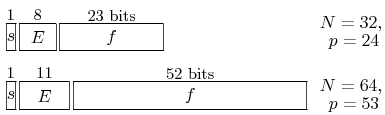
¶ IEEE Standard
The current standard is the ANSI/IEEE Standard 754; see
IEEE (1985, §§1–4). In the case of normalized
binary representation the memory positions for single precision
(![]() ,
, ![]() ,
, ![]() ,
, ![]() ) and
double precision (
) and
double precision (![]() ,
, ![]() ,
, ![]() ,
,
![]() ) are as in Figure 3.1.1. The
respective machine precisions are
) are as in Figure 3.1.1. The
respective machine precisions are
![]() and
and
![]() .
.

- Symbols:
-
: sign, : number of significant bits, : exponent,
 : fractional part and
  : number of bits in floating point
- Referenced by:
- ¶ ‣ §3.1(i)
- Permalink:
- http://dlmf.nist.gov/3.1.F1
- Encodings:
- TeX, png
¶ Rounding
Let ![]() be any positive number with
be any positive number with
- Symbols:
-
: bit, : number of significant bits and : exponent
- Permalink:
- http://dlmf.nist.gov/3.1.E4
- Encodings:
- TeX, pMML, png
![]() , and
, and
- Symbols:
-
: bit, : number of significant bits, : exponent and
 : machine epsilon
- Permalink:
- http://dlmf.nist.gov/3.1.E5
- Encodings:
- TeX, TeX, pMML, pMML, png, png
Then rounding by chopping or rounding down of ![]() gives
gives ![]() ,
with maximum relative error
,
with maximum relative error ![]() . Symmetric rounding or
rounding to nearest of
. Symmetric rounding or
rounding to nearest of ![]() gives
gives ![]() or
or ![]() , whichever is nearer
to
, whichever is nearer
to ![]() , with maximum relative error equal to the machine precision
, with maximum relative error equal to the machine precision
![]() .
.
Negative numbers ![]() are rounded in the same way as
are rounded in the same way as ![]() .
.
§3.1(ii) Interval Arithmetic
- Keywords:
- arithmetics, interval, interval arithmetic, validated computing
- Permalink:
- http://dlmf.nist.gov/3.1.ii
Interval arithmetic is intended for bounding the total effect of rounding errors of calculations with machine numbers. With this arithmetic the computed result can be proved to lie in a certain interval, which leads to validated computing with guaranteed and rigorous inclusion regions for the results.
Let ![]() be the set of closed intervals
be the set of closed intervals ![]() . The elementary arithmetical
operations on intervals are defined as follows:
. The elementary arithmetical
operations on intervals are defined as follows:
- Symbols:
-
 : element of and
  : set of closed intervals
- Permalink:
- http://dlmf.nist.gov/3.1.E6
- Encodings:
- TeX, pMML, png
where ![]() , with appropriate roundings of the end points of
, with appropriate roundings of the end points of
![]() when machine numbers are being used. Division is possible only if the
divisor interval does not contain zero.
when machine numbers are being used. Division is possible only if the
divisor interval does not contain zero.
§3.1(iii) Rational Arithmetics
- Keywords:
- arithmetics, exact rational arithmetic, rational arithmetics
- Permalink:
- http://dlmf.nist.gov/3.1.iii
Computer algebra systems use exact rational arithmetic with rational
numbers ![]() , where
, where ![]() and
and ![]() are multi-length integers. During the
calculations common divisors are removed from the rational numbers, and the
final results can be converted to decimal representations of arbitrary length.
For further information see Matula and Kornerup (1980).
are multi-length integers. During the
calculations common divisors are removed from the rational numbers, and the
final results can be converted to decimal representations of arbitrary length.
For further information see Matula and Kornerup (1980).
§3.1(iv) Level-Index Arithmetic
- Keywords:
- arithmetics, generalized logarithms, generalized precision, level-index arithmetic
- Referenced by:
- §4.44
- Permalink:
- http://dlmf.nist.gov/3.1.iv
To eliminate overflow or underflow in finite-precision arithmetic numbers are
represented by using generalized logarithms ![]() given by
given by
- Symbols:
-
 : principal branch of logarithm function and
  : base
- Permalink:
- http://dlmf.nist.gov/3.1.E7
- Encodings:
- TeX, TeX, pMML, pMML, png, png
with ![]() and
and ![]() the unique nonnegative integer such that
the unique nonnegative integer such that
![]() . In level-index arithmetic
. In level-index arithmetic ![]() is
represented by
is
represented by ![]() (or
(or ![]() for negative numbers).
Also in this arithmetic generalized precision can be defined, which includes
absolute error and relative precision (§3.1(v)) as special cases.
for negative numbers).
Also in this arithmetic generalized precision can be defined, which includes
absolute error and relative precision (§3.1(v)) as special cases.
§3.1(v) Error Measures
- Keywords:
- absolute error, arithmetics, error measures, mollified error, relative error, relative precision
- Referenced by:
- §3.1(iv)
- Permalink:
- http://dlmf.nist.gov/3.1.v
If ![]() is an approximation to a real or complex number
is an approximation to a real or complex number ![]() , then the
absolute error is
, then the
absolute error is
- Symbols:
 : absolute error
- A&S Ref:
- 3.5.1 (in absolute value)
- Permalink:
- http://dlmf.nist.gov/3.1.E8
- Encodings:
- TeX, pMML, png
If ![]() , the relative error is
, the relative error is
- Symbols:
-
: absolute error and
 : relative error
- A&S Ref:
- 3.5.2 (in absolute value)
- Permalink:
- http://dlmf.nist.gov/3.1.E9
- Encodings:
- TeX, pMML, png
The relative precision is
- Symbols:
-
: principal branch of logarithm function and
 : relative precision
- Permalink:
- http://dlmf.nist.gov/3.1.E10
- Encodings:
- TeX, pMML, png
where ![]() for real variables, and
for real variables, and ![]() for complex
variables (with the principal value of the logarithm).
for complex
variables (with the principal value of the logarithm).
The mollified error is
- Symbols:
-
 : open interval and
  : molified error
- Permalink:
- http://dlmf.nist.gov/3.1.E11
- Encodings:
- TeX, pMML, png
For error measures for complex arithmetic see Olver (1983).