

§14.30 Spherical and Spheroidal Harmonics
- Keywords:
- Ferrers functions, spherical harmonics, spheroidal harmonics
- Referenced by:
- ¶ ‣ §1.17(iii), ¶ ‣ §18.38(ii), §34.3(vii)
- Permalink:
- http://dlmf.nist.gov/14.30
Contents
§14.30(i) Definitions
- Notes:
- See Edmonds (1974, p. 24).
- Keywords:
- sectorial harmonics, spherical harmonics, spheroidal harmonics, surface harmonics of the first kind, tesseral harmonics
- Referenced by:
- §10.73(ii)
- Permalink:
- http://dlmf.nist.gov/14.30.i
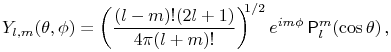
With ![]() and
and ![]() integers such that
integers such that ![]() , and
, and ![]() and
and ![]() angles such that
angles such that ![]() ,
, ![]() ,
,
- Defines:
 : spherical harmonic
- Symbols:
-
 : Ferrers function of the first kind,
  : cosine function,
  : base of exponential function,
  :
:  : factorial,
  : nonnegative integer and
  : nonnegative integer
- Referenced by:
- §14.30(i), §14.30(ii), §14.30(ii), §14.30(iv)
- Permalink:
- http://dlmf.nist.gov/14.30.E1
- Encodings:
- TeX, pMML, png
- Defines:
 : surface harmonic of the first kind
- Symbols:
-
: Ferrers function of the first kind, : cosine function,
 : sine function, : nonnegative integer and : nonnegative integer
- Permalink:
- http://dlmf.nist.gov/14.30.E2
- Encodings:
- TeX, pMML, png
![]() are known as spherical
harmonics.
are known as spherical
harmonics. ![]() are known as surface
harmonics of the first kind: tesseral for
are known as surface
harmonics of the first kind: tesseral for ![]() and sectorial
for
and sectorial
for ![]() . Sometimes
. Sometimes ![]() is denoted by
is denoted by
![]() ; also the definition of
; also the definition of
![]() can differ from
(14.30.1), for example, by inclusion of a factor
can differ from
(14.30.1), for example, by inclusion of a factor
![]() .
.
![]() and
and ![]() (
(![]() ) are often referred
to as the prolate spheroidal harmonics of the first and second kinds,
respectively.
) are often referred
to as the prolate spheroidal harmonics of the first and second kinds,
respectively. ![]() and
and ![]() (
(![]() ) are
known as oblate spheroidal harmonics of the first and second kinds,
respectively. Segura and Gil (1999) introduced the scaled oblate spheroidal
harmonics
) are
known as oblate spheroidal harmonics of the first and second kinds,
respectively. Segura and Gil (1999) introduced the scaled oblate spheroidal
harmonics ![]() and
and
![]() which are real when
which are real when ![]() and
and ![]() .
.
§14.30(ii) Basic Properties
- Notes:
- For (14.30.3), (14.30.6), and
(14.30.8) see Edmonds (1974, pp. 20–21).
(Note that Edmonds’
 differs by a factor
  from
from
 .)
(14.30.4) may be derived from (14.8.1),
(14.8.2), and (14.30.1).
(14.30.5) may be derived from (14.5.1) and
(14.30.1).
(14.30.7) may be derived from (14.7.17) and
(14.30.1).
(14.30.3) also follows from
(14.30.1) and (14.7.10).
.)
(14.30.4) may be derived from (14.8.1),
(14.8.2), and (14.30.1).
(14.30.5) may be derived from (14.5.1) and
(14.30.1).
(14.30.7) may be derived from (14.7.17) and
(14.30.1).
(14.30.3) also follows from
(14.30.1) and (14.7.10). - Keywords:
- spherical harmonics
- Permalink:
- http://dlmf.nist.gov/14.30.ii
Most mathematical properties of ![]() can
be derived directly from (14.30.1) and the properties
of the Ferrers function of the first kind given earlier in this chapter.
can
be derived directly from (14.30.1) and the properties
of the Ferrers function of the first kind given earlier in this chapter.
¶ Explicit Representation

- Symbols:
-
: cosine function,
 : derivative of
  with respect to
  , : base of exponential function, : : factorial, : sine function, : spherical harmonic, : nonnegative integer and : nonnegative integer
- Referenced by:
- §14.30(ii)
- Permalink:
- http://dlmf.nist.gov/14.30.E3
- Encodings:
- TeX, pMML, png
¶ Special Values

- Symbols:
-
: spherical harmonic, : nonnegative integer and : nonnegative integer
- Referenced by:
- §14.30(ii)
- Permalink:
- http://dlmf.nist.gov/14.30.E4
- Encodings:
- TeX, pMML, png

- Symbols:
-
 : element of, : base of exponential function, : : factorial,
  : set of all integers,
  : not an element of, : spherical harmonic, : nonnegative integer and : nonnegative integer
- Referenced by:
- §14.30(ii)
- Permalink:
- http://dlmf.nist.gov/14.30.E5
- Encodings:
- TeX, pMML, png
¶ Symmetry
- Symbols:
-
: spherical harmonic, : nonnegative integer and : nonnegative integer
- Referenced by:
- §14.30(ii)
- Permalink:
- http://dlmf.nist.gov/14.30.E6
- Encodings:
- TeX, pMML, png
¶ Parity Operation
- Symbols:
-
: spherical harmonic, : nonnegative integer and : nonnegative integer
- Referenced by:
- §14.30(ii)
- Permalink:
- http://dlmf.nist.gov/14.30.E7
- Encodings:
- TeX, pMML, png
¶ Orthogonality
- Symbols:
-
 : Kronecker delta,
  : differential of ,
  : integral, : sine function, : spherical harmonic, : nonnegative integer and : nonnegative integer
- Referenced by:
- §14.30(ii)
- Permalink:
- http://dlmf.nist.gov/14.30.E8
- Encodings:
- TeX, pMML, png
here and elsewhere in this section the asterisk (*) denotes complex conjugate.
§14.30(iii) Sums
- Notes:
- See Edmonds (1974, p. 63).
- Keywords:
- spherical harmonics
- Permalink:
- http://dlmf.nist.gov/14.30.iii
¶ Distributional Completeness
For a series representation of the product of two Dirac deltas in terms of products of spherical harmonics see §1.17(iii).
¶ Addition Theorem

- Symbols:
-
: Ferrers function of the first kind, : cosine function, : sine function, : spherical harmonic, : nonnegative integer and : nonnegative integer
- Referenced by:
- ¶ ‣ §18.18(ii)
- Permalink:
- http://dlmf.nist.gov/14.30.E9
- Encodings:
- TeX, pMML, png
§14.30(iv) Applications
- Notes:
- See Edmonds (1974, pp. 21–22).
- Keywords:
- Ferrers functions, Laplace’s equation, angular momentum operator, geophysics, homogeneous harmonic polynomials, reduced Planck’s constant, spherical coordinates, spherical harmonics
- Referenced by:
- ¶ ‣ §1.5(ii)
- Permalink:
- http://dlmf.nist.gov/14.30.iv
In general, spherical harmonics are defined as the class of homogeneous
harmonic polynomials.
See Andrews et al. (1999, Chapter 9). The special
class of spherical harmonics ![]() ,
defined by (14.30.1), appear in many physical
applications. As an example, Laplace’s equation
,
defined by (14.30.1), appear in many physical
applications. As an example, Laplace’s equation ![]() in spherical
coordinates (§1.5(ii)):
in spherical
coordinates (§1.5(ii)):
- Symbols:
-
 : partial derivative of with respect to , : sine function and
  : solution
- Permalink:
- http://dlmf.nist.gov/14.30.E10
- Encodings:
- TeX, pMML, png
has solutions ![]() , which are everywhere one-valued
and continuous.
, which are everywhere one-valued
and continuous.
In the quantization of angular momentum the spherical harmonics
![]() are normalized solutions of the
eigenvalue equation
are normalized solutions of the
eigenvalue equation
- Symbols:
-
: spherical harmonic, : nonnegative integer, : nonnegative integer and
 : angular momentum operator
- Permalink:
- http://dlmf.nist.gov/14.30.E11
- Encodings:
- TeX, pMML, png
where ![]() is the reduced Planck’s constant, and
is the reduced Planck’s constant, and ![]() is the angular
momentum operator in spherical coordinates:
is the angular
momentum operator in spherical coordinates:
- Symbols:
-
: partial derivative of with respect to , : sine function and : angular momentum operator
- Permalink:
- http://dlmf.nist.gov/14.30.E12
- Encodings:
- TeX, pMML, png
see Edmonds (1974, §2.5).
For applications in geophysics see Stacey (1977, §§4.2, 6.3, and 8.1).