
Working with BAM Files
Step 1: Introduction
This tutorial will take you through the several scenarios demonstrating BAM files in Genome Workbench. The 4 scenarios demonstrated are:
- A sorted BAM file with index and coverage graph
- A sorted BAM file with index and no coverage graph
- A sorted BAM file with no index and no coverage graph
- A unsorted BAM file with no index and no coverage graph
The last two examples require you to have SAMTools installed and available. SAMTools can be downloaded here:
http://samtools.sourceforge.net
Since BAM files can be VERY large, they are not loaded into the gBench project as other types of data and exist externally. Example files for this tutorial can be downloaded here (note the file is large ~365MB):
Step 2: Getting Started

From the File menu choose Open and select BAM files from the left side.
Select button on the right that says Add a BAM file. Navigate
to the BAM Test Files folder you downloaded select

with_index_with_graph. Click Open, select mapt.NA12156.altex.bam and click Open. Click Next three times and then click Finish.
Now there's a 'New Project' in the Project Tree View. Double click mapt.NA12156.altex (coverage graph) to open the Open View dialog. Double click the Graphical View. Select the second row (the one that starts with NT) in the Converted Object dialog and click Finish. You can optionally choose the row that starts with NC, but the graph is less interesting.
Depending on your settings, if you don't see the alignments in the graphical view, you'll have to turn them on by clicking on the Content Menu (see figure) and choosing Alignments.
Step 3: Viewing the BAM Data
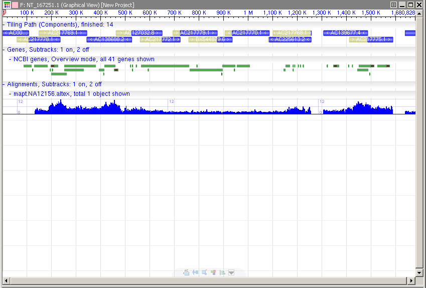
Now you should have a track in the graphical view titled "mapt.NA12156.altex" and it's a blue graph. All the standard Genome Workbench navigation tools are available for panning and zooming (see Tutorial 1). 
If you zoom in far enough, you'll see the coverage graph change to show the alignments.
And if you zoom in even further, you'll see the sequence with insertions and deletions highlighted.
Step 4: BAM file with no coverage graph
The steps for this part are identical to Steps 1 and 2 in this tutorial, however with a different data file.
From the File menu choose Open and select BAM files from the left side.
Select button on the right that says Add a BAM file. Navigate to the BAM Test Files folder you downloaded select with_index_no_graph. Click Open, select mapt.NA12156.altex.bam and click Open. Click Next three times and then click Finish.
Now there's a 'New Project' in the Project Tree View. Double click mapt.NA12156.altex coverage graph (note the name of the data is slightly different than the first exercise) to open the Open View dialog. Double click the Graphical View. Select the second row (the one that starts with NT) in the Converted Object dialog and click Finish. You can optionally choose the row that starts with NC, but the graph is less interesting.
Depending on your settings, if you don't see the alignments in the graphical view, you'll have to turn them on by clicking on the Content Menu (see figure) and choosing Alignments.
Step 5: Viewing the BAM Data
The steps for this part are identical to Steps 1 and 2 in this tutorial, however with a different data file.
Now you should have a track in the graphical view titled "mapt.NA12156.altex" and it's a blue graph. All the standard Genome Workbench navigation tools are available for panning and zooming (see Tutorial 1, steps 6,).
If you zoom in far enough, you'll see the coverage graph change to show the alignments.
And if you zoom in even further, you'll see the sequence with insertions and deletions highlighted.
Step 6: BAM file with no index and no coverage graph
This exercise requires the presence of SAMTools - freely available package for working with BAM files. Download and expand the package and put it in a convenient folder/directory.
Then the steps are similar to Exercises 1 and 2. From the File menu choose Open and select BAM files from the left side. Select button on the right that says Add a BAM file.
Navigate to the BAM Test Files folder you downloaded select no_index_no_graph_sorted.
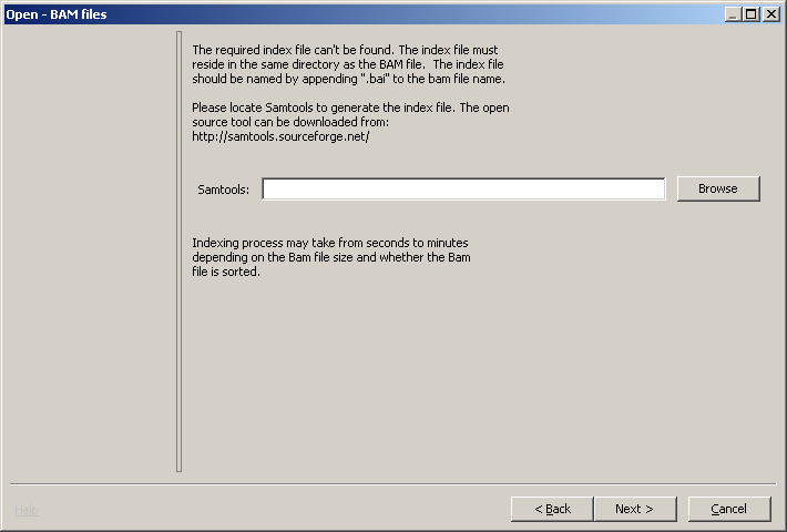
Since there is no index file for this BAM file we need SAMTools to create one. You'll see the dialog shown, gBench asking where to find the SAMTools executable. When you navigate to SAMTools on your computer click Open and then Next 3 times. Click Open, select mapt.NA12156.altex.bam and click Open. Click Next three times and then click Finish. Once you've done this, it's just like step 1.
Now there's a 'New Project' in the Project Tree View. Double click mapt.NA12156.altex (coverage graph) to open the Open View dialog. Double click the Graphical View. Select the second row (the one that starts with NT) in the Converted Object dialog and click Finish. You can optionally choose the row that starts with NC, but the graph is less interesting.
Depending on your settings, if you don't see the alignments in the graphical view, you'll have to turn them on by clicking on the Content Menu (see figure) and choosing Alignments.
Step 7: Viewing the BAM Data
The steps for this part are identical to Steps 1 and 2 in this tutorial, however with a different data file.
Now you should have a track in the graphical view titled "mapt.NA12156.altex" and it's a blue graph. All the standard Genome Workbench navigation tools are available for panning and zooming (see Tutorial 1, steps 6, 7 and 8).
If you zoom in far enough, you'll see the coverage graph change to show the alignments.
And if you zoom in even further, you'll see the sequence with insertions and deletions highlighted.
Step 8: Unsorted BAM file with no index and no coverage graph
This exercise requires the presence of SAMTools - freely available package for working with BAM files. Download and expand the package and put it in a convenient folder/directory.
Then the steps are similar to
Exercises 1 and 2. From the File menu choose Open and select BAM files from the left side. Select button on the right that says Add a BAM file. Navigate to the BAM Test Files folder you downloaded select no_index_no_graph_unsorted_need_id_mapping.
Since there is no index file for this BAM file we need SAMTools to create one. You'll see the dialog shown, gBench asking where to find the SAMTools executable. When you navigate to SAMTools on your computer click Open and then Next 3 times. Click Open, select GSM409307_UCSD.H3K4me1.bam and click Open. Click Next twice. When you get the Id Mapping Context page, select hg18 - NCBI Human build 36 and click Next. Then click Finish.
SAMTools can take several minutes to process this data
Once you've done this, it's similar to step 1.
There's a 'New Project' in the Project Tree View. Double click GSM409307_UCSD.H3K4.me1.sorted coverage graph to open the Open View dialog. Double click the Graphical View. Select NC_000020.0 (see figure) in the Converted Object dialog and click Finish. You can choose any row but there may be no graph data. Click Ok when you're told there's a newer version.
Depending on your settings, if you don't see the alignments in the graphical view, you'll have to turn them on by clicking on the Content Menu (see figure) and choosing Alignments.
Step 9: Viewing the BAM Data
The steps for this part are identical to Steps 1 and 2 in this tutorial, however with a different data file.
Now you should have a track in the graphical view titled "GSM409307_UCSD.H3K4me1.bam.sorted" and it's a blue graph. All the standard Genome Workbench navigation tools are available for panning and zooming (see Tutorial 1).
If you zoom in far enough, you'll see the coverage graph change to show the alignments.
And if you zoom in even further, you'll see the sequence with insertions and deletions highlighted.
Step 10:Finished!
Congratulations! You now know how open and manipulate several different flavors of BAM files in Genome Workbench.
Download
Current Version is 2.6.0 (released August 31, 2012)
- Release Notes
- Windows
- Mac OS X
- Linux (Ubuntu 10.04 LTS (Lucid Lynx))
- Source
- Older Versions