SOURCE OF DATA
The data in this microdata file come from the June 2000 Current Population Survey (CPS). The June survey uses two sets of questions, the basic CPS and the supplement.
Basic CPS. The basic CPS collects primarily labor force data about the civilian noninstitutional population. Interviewers ask questions concerning labor force participation about each member 15 years old and over in every sample household.
June 2000 Supplement. In addition to the basic CPS questions, interviewers asked supplementary questions in June 2000 about fertility of women between 15 and 44 years of age.
Sample design. The present CPS sample was selected from the 1990 Decennial Census files with coverage in all 50 states and the District of Columbia. The sample is continually updated to account for new residential construction. To obtain the sample, the United States was divided into 2,007 geographic areas. In most states, a geographic area consisted of a county or several contiguous counties. In some areas of New England and Hawaii, minor civil divisions are used instead of counties. These 2,007 geographic areas were then grouped into 754 strata, and one geographic area was selected from each stratum. About 50,000 occupied households are eligible for interview every month out of these 754 areas. Interviewers are unable to obtain interviews at about 3,200 of these units. This occurs when the occupants are not found at home after repeated calls or are unavailable for some other reason.
Sample Redesign. Since the introduction of the CPS, the Census Bureau has redesigned the CPS sample several times. These redesigns have improved the quality and accuracy of the data and have satisfied changing data needs. The most recent changes were completely implemented in July 1995.
Estimation procedure. This survey's estimation procedure adjusts weighted sample results to agree with independent estimates of the civilian noninstitutional population of the United States by age, sex, race, Hispanic/non-Hispanic origin, and state of residence. The adjusted estimate is called the post-stratification ratio estimate. The independent estimates are calculated based on information from four primary sources:
The independent population estimates include some, but not all, undocumented immigrants.
ACCURACY OF THE ESTIMATES
A sample survey estimate has two possible types of error: sampling and nonsampling. The accuracy of an estimate depends on both types of error. The nature of the sampling error is known given the survey design. The full extent of the nonsampling error, however, is unknown.
Sampling Error. Since the CPS estimates come from a sample, they may differ from figures from a complete census using the same questionnaires, instructions, and enumerators. This possible variation in the estimates due to sampling error is known as "sampling variability."
Consequently, one should be particularly careful when interpreting results based on a relatively small number of cases or on small differences between estimates. The standard errors for CPS estimates primarily indicate the magnitude of sampling error. They also partially measure the effect of some nonsampling errors in responses and enumeration, but do not measure systematic biases in the data. (Bias is the average over all possible samples of the differences between the sample estimates and the desired value.)
Nonsampling Error. All other sources of error in the survey estimates are collectively called nonsampling error. Sources of nonsampling errors include the following:
Nonresponse. The effect of nonresponse cannot be measured directly, but one indication of its potential effect is the nonresponse rate. For the June 2000 basic CPS, the nonresponse rate was 7.1%. The nonresponse rate for the Fertility supplement was an additional 4.9%, for a total supplement nonresponse rate of 11.6%.
Coverage. The concept of coverage in the survey sampling process is the extent to which the total population that could be selected for sample covers the survey's target population. CPS undercoverage results from missed housing units and missed persons within sample households. Overall CPS undercoverage is estimated to be about 8 percent. CPS undercoverage varies with age, sex, and race. Generally, undercoverage is larger for males than for females and larger for Blacks and other races combined than for Whites. As described previously, ratio estimation to independent age-sex-race-Hispanic population controls partially corrects for the bias due to undercoverage. However, biases exist in the estimates to the extent that missed persons in missed households or missed persons in interviewed households have different characteristics from those of interviewed persons in the same age-sex-race-origin-state group.
A common measure of survey coverage is the coverage ratio, the estimated population before post-stratification divided by the independent population control. Table A shows CPS coverage ratios for age-sex-race groups for a typical month. The CPS coverage ratios can exhibit some variability from month to month. Other Census Bureau household surveys experience similar coverage.
| Non-Black | Black | All Persons | |||||
|---|---|---|---|---|---|---|---|
| Age | M | F | M | F | M | F | Total |
| 0-14 | 0.929 | 0.964 | 0.850 | 0.838 | 0.916 | 0.943 | 0.929 |
| 15 | 0.933 | 0.895 | 0.763 | 0.824 | 0.905 | 0.883 | 0.895 |
| 16-19 | 0.881 | 0.891 | 0.711 | 0.802 | 0.855 | 0.877 | 0.866 |
| 20-29 | 0.847 | 0.897 | 0.660 | 0.811 | 0.823 | 0.884 | 0.854 |
| 30-39 | 0.904 | 0.931 | 0.680 | 0.845 | 0.877 | 0.920 | 0.899 |
| 40-49 | 0.928 | 0.966 | 0.816 | 0.911 | 0.917 | 0.959 | 0.938 |
| 50-59 | 0.953 | 0.974 | 0.896 | 0.927 | 0.948 | 0.969 | 0.959 |
| 60-64 | 0.961 | 0.941 | 0.954 | 0.953 | 0.960 | 0.942 | 0.950 |
| 65-69 | 0.919 | 0.972 | 0.982 | 0.984 | 0.924 | 0.973 | 0.951 |
| 70+ | 0.993 | 1.004 | 0.996 | 0.979 | 0.993 | 1.002 | 0.998 |
| 15+ | 0.914 | 0.945 | 0.767 | 0.874 | 0.898 | 0.927 | 0.918 |
| 0+ | 0.918 | 0.949 | 0.793 | 0.864 | 0.902 | 0.931 | 0.921 |
A Nonsampling Error Warning. Since the full extent of the nonsampling error is unknown, one should be particularly careful when interpreting results based on small differences between estimates. Even a small amount of nonsampling error can cause a borderline difference to appear significant or not, thus distorting a seemingly valid hypothesis test. Caution should also be used when interpreting results based on a relatively small number of cases. Summary measures probably do not reveal useful information when computed on a base1 smaller than 75,000. For additional information on nonsampling error including the possible impact on CPS data when known, refer to Statistical Policy Working Paper 3, An Error Profile: Employment as Measured by the Current Population Survey, Office of Federal Statistical Policy and Standards, U.S. Department of Commerce, 1978 and Technical Paper 63, The Current Population Survey: Design and Methodology, Bureau of the Census, U.S. Department of Commerce.
Standard Errors and Their Use. The sample estimate and its standard error enable one to construct a confidence interval. A confidence interval is a range that would include the average result of all possible samples with a known probability. For example, if all possible samples were surveyed under essentially the same general conditions and using the same sample design, and if an estimate and its standard error were calculated from each sample, then approximately 90 percent of the intervals from 1.645 standard errors below the estimate to 1.645 standard errors above the estimate would include the average result of all possible samples.
A particular confidence interval may or may not contain the average estimate derived from all possible samples. However, one can say with specified confidence that the interval includes the average estimate calculated from all possible samples.
Standard errors may also be used to perform hypothesis testing. This is a procedure for distinguishing between population parameters using sample estimates. The most common type of hypothesis is that the population parameters are different. An example of this would be comparing the percentage of women between 15 and 44 years of age who had a child in 2000 that were in the labor force to the percentage of women between 15 and 44 years of age who had a child in 1998 that were in the labor force. An illustration of this is included in the following pages.
Tests may be performed at various levels of significance. A significance level is the probability of concluding that the characteristics are different when, in fact, they are the same. To conclude that two parameters are different at the 0.10 level of significance, the absolute value of the estimated difference between characteristics must be greater than or equal to 1.645 times the standard error of the difference.
The Census Bureau uses 90-percent confidence intervals and 0.10 levels of significance to determine statistical validity. Consult standard statistical textbooks for alternative criteria.
Standard errors of estimated numbers. The approximate standard error, sx, of an estimated number from this microdata file can be obtained using this formula:
| Formula (1) |
Here x is the size of the estimate and a and b are the parameters in Table 2 or 3 associated with the particular type of characteristic. When calculating standard errors from cross-tabulations involving different characteristics, use the set of parameters for the characteristic which will give the largest standard error.
Illustration
Suppose there were 563,000 unemployed women 35-44 years of age in the civilian labor force. Use the appropriate parameters from Table 2 and Formula (1) to get
| Number, x a parameter b parameter Standard error 90% conf. int. |
563000 -0.000018 2,957 41,000 496,000 to 630,000 |
The standard error is calculated as
![]()
the 90-percent confidence interval is calculated as 563,000 ± 1.645 x 41,000.
A conclusion that the average estimate derived from all possible samples lies within a range computed in this way would be correct for roughly 90 percent of all possible samples.
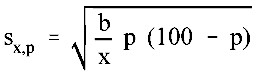
Standard Errors of Estimated Percentages. The reliability of an estimated percentage, computed using sample data for both numerator and denominator, depends on the size of the percentage and its base. Estimated percentages are relatively more reliable than the corresponding estimates of the numerators of the percentages, particularly if the percentages are 50 percent or more. When the numerator and denominator of the percentage are in different categories, use the parameter from Table 2 or 3 indicated by the numerator.
The approximate standard error, sx,p, of an estimated percentage can be obtained by use of the formula
 |
| Formula (2) |
Here x is the total number of persons, families, households, or unrelated individuals in the base of the percentage, p is the percentage (0 ≤ p ≤ 100), and b is the parameter in Table 2 or 3 associated with the characteristic in the numerator of the percentage.
Illustration.
Suppose that 6.5 percent of the 60,873,000 women 15-44 years old had a child in the last year. Use the appropriate parameter from Table 3 and formula (2) to get
| Percentage, p Base, x b parameter Standard error 90% conf. int. |
6.5 60,873,000 2,241 0.15 6.3 to 6.7 |
The standard error is calculated as
The 90-percent confidence interval for the percentage of women 15-44 years old who had a child in the last year is calculated as 6.5 ± 1.645x0.15.
Standard Error of a Difference. The standard error of the difference between two sample estimates is approximately equal to
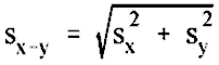 |
| Formula (3) |
where sx and sy are the standard errors of the estimates, x and y. The estimates can be numbers, percentages, ratios, etc. This will represent the actual standard error quite accurately for the difference between estimates of the same characteristic in two different areas, or for the difference between separate and uncorrelated characteristics in the same area. However, if there is a high positive (negative) correlation between the two characteristics, the formula will overestimate (underestimate) the true standard error.
Illustration
Suppose that of 3,934,000 women in 2000 between 15-44 years of age who had a child in the previous year, 2,170,000 or 55.2 percent were in the labor force, and of the 3,671,000 women in 1998 between 15-44 years of age who had a child in the previous year, 2,155,000 or 58.7 percent were in the labor force. Use the appropriate parameters from Table 2 and formulas (3) and (4) to get
| x | y | difference | |
| Percentage Base b parameter Standard error 90% conf. int. |
55.2 3,934,000 2,530 1.26 53.1 to 57.3 |
58.7 3,671,000 2,530 1.29 56.6 to 60.8 |
3.5 - - 1.80 0.5 to 6.5 |
The standard error of the difference is calculated as
The 90-percent confidence interval around the difference is calculated as 3.5 ± 1.645 x 1.80. Since this interval does not include zero, we can conclude with 90 percent confidence that the percentage of women between 15-44 years of age who had a child in 2000 who were in the labor force is different from the percentage of women between 15-44 years of age who had a child in 1998 who were in the labor force.
Standard error of a fertility ratio. The standard error of a fertility ratio is a function of the number of children ever born per 1,000 women and the number of women in a given category. The formula for the standard error of a fertility ratio is
 |
| Formula (4) |
where a, b and c are the parameters from Table 4, x is the number of children ever born or expected per 1,000 women and y is the number of women, in thousands. This formula should be used when calculating standard errors for estimates involving the possibility of more than one event per woman, i.e., number of children ever born. For data involving at most one event per woman, convert the ratio to a percentage and use formula (2) and the parameters in Table 2 or 3 to calculate the standard errors.
Illustration.
Suppose that 10,055,000 ever-married women 40-44 years old had 2,050 children ever born per 1,000 women. Use formula (4) and the parameters in Table 4 to get
| Children Ever Born, x Base, 1,000y a parameter b parameter c parameter Standard error 90% conf. int. |
2,050 10,055,000 +0.0000014 901 1,644 30 2,001 to 2,099 |
The standard error is calculated as
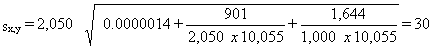
The 90-percent confidence interval is from 2,001 to 2,099 children ever born per 1,000 women (i.e., 2,050 ± 1.645 x 30). A conclusion that the average estimate derived from all possible samples lies within a range computed in this way would be correct for roughly 90 percent of all possible samples.
Standard Error of a Ratio. Certain estimates may be calculated as the ratio of two numbers.
The standard error of a ratio, x/y, may be computed using
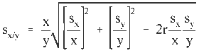 |
| Formula (5) |
The standard error of the numerator, sx, and that of the denominator, sy, may be calculated using formulas described earlier. In formula (5), r represents the correlation between the numerator and the denominator of the estimate.
For one type of ratio, the denominator is a count of families or households and the numerator is a count of persons in those families or households with a certain characteristic. If there is at least one person with the characteristic in every family or household, use 0.7 as an estimate of r. An example of this type is the mean number of children per family with children.
For all other types of ratios, r is assumed to be zero. If r is actually positive (negative), then this procedure will provide an overestimate (underestimate) of the standard error of the ratio. Examples of this type are the mean number of children per family and the poverty rate.
NOTE: For estimates expressed as the ratio of x per 100 y or x per 1,000 y, multiply formula (5) by 100 or 1,000, respectively, to obtain the standard error.
Illustration.
Suppose there are 35,778,000 ever-married women 15-44 years old and 25,095,000 never-married women 15-44 years old. The ratio of ever-married women, x, to never-married women, y, is 1.43. Use the appropriate parameters from Table 3 and equations (1) and (5) to get
| x | y | ratio | |
| Estimate | 35,778,000 | 25,095,000 | 1.43 |
| a parameter | -0.000024 | -0.000024 | - |
| b parameter | 5,211 | 5,211 | - |
| Standard error | 395,000 | 340,000 | 0.02 |
| 90% conf. int. | 35,128,000 to 36,428,000 |
24,536,000 to 25,654,000 |
1.40 to 1.46 |
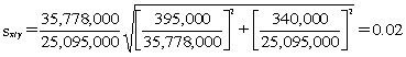
Using formula (5) with r = 0, the estimate of the standard error is
The 90-percent confidence interval is calculated as 1.43 ±1.645x0.02.
Standard errors for region, state and nonmetropolitan estimates. Multiply the parameters in Tables 2, 3 and 4 by the factors in Tables 5 and 6 to get state, region and nonmetropolitan parameters for labor force and fertility estimates.
| Characteristic | a | b |
|---|---|---|
| Labor Force and Not In Labor Force Data Other than Agricultural Employment and Unemployment | ||
| Total 1 | -0.000018 | 2,985 |
| Men 1 | -0.000033 | 2,764 |
| Women | -0.000030 | 2,530 |
| Both sexes, 16 to 19 years | -0.000172 | 2,545 |
| White 1 | -0.000020 | 2,985 |
| Men | -0.000037 | 2,767 |
| Women | -0.000034 | 2,527 |
| Both sexes, 16 to 19 years | -0.000204 | 2,550 |
| Black | -0.000125 | 3,139 |
| Men | -0.000302 | 2,931 |
| Women | -0.000183 | 2,637 |
| Both sexes, 16 to 19 years | -0.001295 | 2,949 |
| Hispanic origin | -0.000206 | 3,896 |
| Not In Labor Force (use only for Total, Total Men, and White) | +0.000006 | 829 |
| Agricultural Employment | ||
| Total or White | +0.000782 | 3,049 |
| Men | +0.000858 | 2,825 |
| Women or Both sexes, 16 to 19 years |
-0.000025 | 2,582 |
| Black | -0.000135 | 3,155 |
| Hispanic origin | ||
| Total or Women | +0.011857 | 2,895 |
| Men or Both sexes, 16 to 19 years |
+0.015736 | 1,703 |
| Unemployment | ||
| Total or White | -0.000018 | 2,957 |
| Black | -0.000212 | 3,150 |
| Hispanic origin | -0.000102 | 3,576 |
NOTE:These parameters are to be applied to basic CPS monthly labor force estimates.
For foreign-born characteristics for Total and White, the a and b parameters should be multiplied by 1.3. No adjustment is necessary for foreign-born characteristics for Blacks and Hispanics.
| Characteristic | People | Households, etc. | ||
|---|---|---|---|---|
| a | b | a | b | |
| FERTILITY1 | ||||
| Total or White | -0.000037 | 2,241 | (X) | (X) |
| Black | -0.000251 | 2,241 | (X) | (X) |
| Hispanic | -0.000450 | 4,100 | (X) | (X) |
| Asian/Pacific Islander | -0.000631 | 2,241 | (X) | (X) |
| NUMBER OF BIRTHS | ||||
| Total or White | -0.000067 | 4,087 | (X) | (X) |
| Black | -0.000457 | 4,081 | (X) | (X) |
| Hispanic | -0.000802 | 7,312 | (X) | (X) |
| Asian/Pacific Islander | -0.001149 | 4,081 | (X) | (X) |
| MARITAL STATUS, HOUSEHOLD & FAMILY CHARACTERISTICS | ||||
| Total or White | -0.000024 | 5,211 | -0.000010 | 2,068 |
| Black | -0.000290 | 7,486 | -0.000072 | 1,871 |
| Hispanic Origin | -0.000551 | 12,616 | -0.000138 | 3,153 |
| Asian/Pacific Islander | -0.000729 | 7,486 | -0.000169 | 1,730 |
| INCOME | ||||
| Total or White | -0.000011 | 2,454 | -0.000010 | 2,241 |
| Black | -0.000109 | 2,810 | -0.000095 | 2,447 |
| Hispanic Origin | -0.000207 | 4,736 | -0.000180 | 4,124 |
| Asian/Pacific Islander | -0.000274 | 2,810 | -0.000238 | 2,447 |
| EDUCATIONAL ATTAINMENT | ||||
| Total or White | -0.000011 | 2,369 | -0.000010 | 2,068 |
| Black | -0.000104 | 2,680 | -0.000072 | 1,871 |
| Hispanic Origin | -0.000133 | 3,052 | -0.000138 | 3,153 |
| Asian/Pacific Islander | -0.000211 | 2,164 | -0.000182 | 1,871 |
| NATIVITY - Born in: | ||||
| Mexico, other North America, South America | -0.000052 | 11,054 | (X) | (X) |
| Europe | -0.000030 | 6,351 | (X) | (X) |
| Asia, Africa, Oceania | -0.000048 | 10,351 | (X) | (X) |
| United States | -0.000024 | 5,211 | (X) | (X) |
1 Fertility includes number of women by number of children ever born, percent childless and women who have had a child in the last year.
Note: For foreign-born characteristics for Total and White, multiply the parameters by 1.3. No adjustments are necessary for Nativity or for foreign born characteristics for Blacks, APIs and Hispanics.
| a | b | c |
|---|---|---|
| +0.0000014 | 901 | 1,644 |
Note: Multiply the parameters by 1.3 to get foreign born parameters
| State | Factor | State | Factor | |
|---|---|---|---|---|
| Alabama | 1.01 | Montana | 0.20 | |
| Alaska | 0.15 | Nebraska | 0.42 | |
| Arizona | 0.97 | Nevada | 0.44 | |
| Arkansas | 0.59 | New Hampshire | 0.38 | |
| California | 1.29 | New Jersey | 0.82 | |
| Colorado | 0.93 | New Mexico | 0.40 | |
| Connecticut | 1.00 | New York | 0.89 | |
| Delaware | 0.22 | North Carolina | 0.94 | |
| District of Columbia | 0.16 | North Dakota | 0.16 | |
| Florida | 0.97 | Ohio | 1.02 | |
| Georgia | 1.40 | Oklahoma | 0.73 | |
| Hawaii | 0.35 | Oregon | 0.86 | |
| Idaho | 0.27 | Pennsylvania | 0.96 | |
| Illinois | 1.00 | Rhode Island | 0.30 | |
| Indiana | 1.38 | South Carolina | 1.01 | |
| Iowa | 0.71 | South Dakota | 0.17 | |
| Kansas | 0.65 | Tennessee | 1.34 | |
| Kentucky | 0.92 | Texas | 1.21 | |
| Louisiana | 0.95 | Utah | 0.43 | |
| Maine | 0.37 | Vermont | 0.18 | |
| Maryland | 1.38 | Virginia | 1.48 | |
| Massachusetts | 0.81 | Washington | 1.47 | |
| Michigan | 0.93 | West Virginia | 0.39 | |
| Minnesota | 1.11 | Wisconsin | 1.23 | |
| Mississippi | 0.64 | Wyoming | 0.12 | |
| Missouri | 1.37 |
| Characteristic | Factor |
| Region | |
| Northeast | 0.85 |
| Midwest | 1.03 |
| South | 1.08 |
| West | 1.09 |
| Nonmetropolitan characteristics | 1.50 |