| Internet: www.bls.gov/ro5/ | FOR IMMEDIATE RELEASE: |
| GENERAL INFORMATION: (312) 353-1880 | Thursday, August 28, 2008 |
| MEDIA CONTACT: Paul LaPorte | |
| (312) 353-1138 |
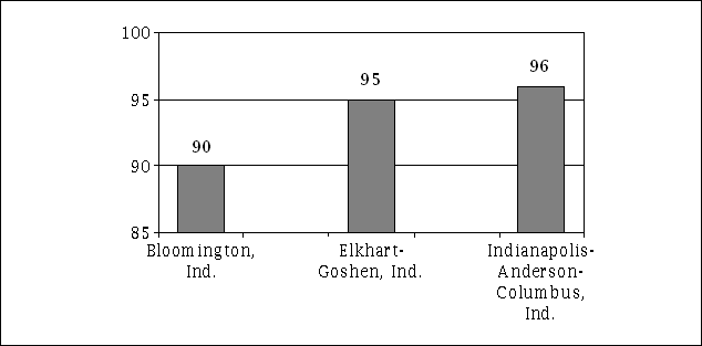
The pay relative averaged across all occupations in the Indianapolis-Anderson-Columbus, Ind. Combined Statistical Area (CSA) was 96 in 2007, meaning that pay on average was 4 percent below the national average. In the Elkhart-Goshen, Ind. and Bloomington, Ind. Metropolitan Statistical Areas (MSAs), the pay relatives were 95 and 90, meaning workers earned on average 5 and 10 percent less than the national average, respectively, according to the U.S. Department of Labor’s Bureau of Labor Statistics (BLS). Regional Commissioner Jay A. Mousa noted that the pay relatives for the three metropolitan areas surveyed in Indiana were all significantly lower than the national average. (See chart A and table A.).
Chart A. Pay relatives for all occupations in metropolitan areas in Indiana, area-to-nation comparisons, National Compensation Survey, July 2007 (U.S. = 100)
BLS produces occupational pay relatives to facilitate comparisons of occupational pay between metropolitan areas and the United States as a whole. Using data from the National Compensation Survey (NCS) pay relatives—a means of assessing relative pay differences—have been prepared for 2007 for each of the 9 major occupational groups with 77 Metropolitan Statistical Areas, as well as averaged across all occupations for each area.
Area-to-Nation Comparisons
In the Indianapolis area, only the production occupational group had a pay relative that was significantly higher than the national average. In contrast, four occupational groups—management, business, and financial; service; office and administrative support; and construction and extraction—posted pay relatives that were significantly lower than the U.S. average. The remaining four occupational groups had pay relatives that were not measurably different from that of the nation.
| Metropolitan Area 1/ |
All Occupations |
Management, business, and financial |
Professional and related |
Service |
Sales and related |
|---|---|---|---|---|---|
United States |
100 | 100 | 100 | 100 | 100 |
Bloomington |
90* | 87* | 92* | 87* | 83* |
Elkhart-Goshen |
95* | 99 | 91* | 97* | 94* |
Indianapolis-Anderson-Columbus |
96* | 79* | 97 | 94* | 94 |
Metropolitan Area 1/ |
Office and administrative support |
Construction and extraction |
Installation, maintenance, and repair |
Production |
Transportation and material moving |
United States |
100 | 100 | 100 | 100 | 100 |
Bloomington |
91* | 76* | 81* | 97 | 105* |
Elkhart-Goshen |
92* | 114* | 89* | 96* | 99 |
Indianapolis-Anderson-Columbus |
96* | 96* | 95 | 106* | 97 |
* The pay relative for this area is significantly different from the national average of all areas at the ten percent level of significance. For additional details, see the Technical Note.
1/ A metropolitan area can be a Metropolitan Statistical Area (MSA) or Combined Statistical Area (CSA) as defined by the Office of Management and Budget, December 2003.
In the Elkhart-Goshen area, the only occupational group to post a significantly higher pay relative was construction and extraction. Six of the nine occupational groups had pay relatives that were significantly below the national average, including office and administrative support and installation, maintenance and repair. The remaining two occupational groups posted pay relatives that were not significantly different from the national average.
Workers in the Bloomington area had significantly different pay relatives than the national average in eight of nine occupational groups. Transportation and material moving was the only occupational group to post a significantly higher pay relative. Seven of the nine occupational groups had pay relatives that were significantly lower than that for the nation, including sales and related jobs, and construction and extraction. The pay relative for the production occupational group did not differ significantly from the national average.
Area-to-Area Comparisons
Area-to-area pay comparisons are useful in determining the difference in pay levels between two metropolitan areas. This type of comparison requires that the base area be changed from the nation to a specific metropolitan area. For example, when the Bloomington area was the base area (pay relative = 100), average pay for all occupational groups in the Indianapolis area was 7 percent higher. (See table 1). When the base area was changed to Elkhart (pay relative = 100), average pay in Bloomington was 6 percent lower and average pay in Indianapolis was not significantly different. (See table 1.)
Area-to-area comparisons are available on the BLS Web site at www.bls.gov/ncs/ocs/payrel.htm.
Area Definitions:
The Bloomington, Ind. Metropolitan Statistical Area is comprised of Greene, Monroe, and Owen Counties in Indiana.
The Elkhart-Goshen, Ind. Metropolitan Statistical Area is comprised of Elkhart County in Indiana.
The Indianapolis-Anderson-Columbus, Ind. Combined Statistical Area is comprised of Bartholomew, Boone, Brown, Hamilton, Hancock, Hendricks, Henry, Jennings, Johnson, Madison, Marion, Montgomery, Morgan, Putnam, and Shelby Counties in Indiana.
What is a pay relative?
A pay relative is a calculation of pay—wages, salaries, commissions, and production bonuses—for a given metropolitan area relative to the nation as a whole. The calculation controls for differences among areas in occupational composition, establishment and occupational characteristics, and the fact that data are collected for areas at different times during the year.
Metropolitan areas often differ greatly in the composition of establishments and occupations that are available to the local workforce. For example, in Brownsville, Texas, the ratio of workers in the high-paying management, business, and financial occupational group to the number of workers in all occupations is under 6 percent, whereas nationally this ratio is over 9 percent 1/. In addition to these factors, the NCS collects compensation data for metropolitan areas at different times during the year. Payroll reference dates differ between areas which makes direct comparisons between areas difficult.
The pay relative approach controls for these differences to isolate the geographic effect on wage determination. To illustrate the importance of controlling for these effects, consider the following example.
The average pay for construction and extraction workers in the New York-Newark-Bridgeport, N.Y.-N.J.-Conn.-Pa. area is $30.42 and the average pay for construction and extraction workers in the entire United States is $20.14 2/. A simple pay comparison can be calculated from the ratio of the two average pay levels, multiplied by 100 to express the comparison as a percentage. The pay comparison in the example is calculated as:
($30.42 ÷ $20.14) * 100 ≅ 151
This comparison does not control for differences between the New York-Newark-Bridgeport area and the nation in the mix of occupations, industries, and other factors. A more accurate estimate of the geographic effect of wages can be obtained by taking these differences into account. Controlling for differences in occupational composition, establishment and occupational characteristics, and the payroll reference date relative to the nation as the whole, the pay relative for construction and extraction occupations in New York-Newark-Bridgeport, N.Y.-N.J.-Conn.-Pa. is equal to 133.
Using pay relative data
To assist data users with the use of these data, tests have been conducted to determine whether differences between each pay relative and the pay relative for the nation as a whole are statistically significant (that is, the pay for the given occupation in that area is too different from the national average to be accounted for by the randomness of the survey’s sample). Similar tests are conducted for the area-to-area comparisons. In all tables, statistically significant pay relatives are denoted with an asterisk (*). More information on significance testing is available in the Technical Note.
Also because of sample variation from year to year, data users are cautioned about inferring that there have been actual changes in underlying economic conditions from changes in the estimated pay relatives between 2006 and 2007. This caution applies even more strongly to estimates by occupational group.
1/ Data for this example are based on the May 2007 Metropolitan and Nonmetropolitan Area Occupational Employment and Wage Estimates, www.bls.gov/oes/current/oessrcma.htm.
2/ Average pay for construction and extraction workers in the New York-Newark-Bridgeport, N.Y.-N.J.-Conn.-Pa. metropolitan area and for the United States are based on wage estimates published in the New York-Newark-Bridgeport, N.Y.-N.J.-Conn.-Pa., National Compensation Survey, May 2007 and the upcoming National Compensation Survey: Occupational Wages in the United States, July 2007, www.bls.gov/ncs/ncswage2007.htm.
Technical Note
Because the NCS is a sample survey, data are subject to sampling error. For the data presented here, sampling errors are differences that occur between the pay relatives estimated from the sample and the true pay relatives derived from the population. It is important to assess whether differences between each pay relative and the pay relative for the nation as a whole is likely to be a result of sampling error or of true differences in pay levels. To perform this assessment, a test of statistical significance is conducted.
The test constructs a 90-percent confidence interval that assumes the given area’s true pay relative is equal to the national average. The confidence interval is constructed so that there is a 90 percent probability the pay relative calculated from any one sample is contained within the confidence interval. If from a single sample a calculated pay relative falls within the confidence interval, then the pay relative is not statistically significant and the hypothesis that the true pay relative is equal to the national average is accepted. However, if the pay relative falls outside of the constructed confidence interval then the pay relative is statistically significant at the 10-percent level. The hypothesis that the given area’s pay relative is equal to the pay relative for the nation is rejected and one can conclude with reasonable confidence that the true pay relative is different from the national average.
In addition to sampling error, pay relatives are subject to a variety of sources that can adversely influence the estimates. The NCS may be unable to obtain information for some establishments; there may be difficulties with survey definitions; respondents may be unable to provide correct information, or mistakes in recording or coding the data may occur. Non-sampling errors of these kinds were not specifically measured. However, they are expected to be minimal due to the extensive training of the field economists who gathered the survey data, computer edits of the data, and detailed data review.
Historical pay relative data are available for 1992-1996, 1998, 2002, 2004-2006. There are several differences between the recent pay relatives and the pay relatives for earlier years, including different industry and occupation classification systems, varying methodology, and different survey designs. These differences limit comparability. The pay relatives for 2004 through 2007 were calculated using the same industry and occupation classification systems, methodology, and survey design. Nonetheless, comparisons between the estimates for the two years should be made only with a high degree of caution.
Pay relatives were estimated using a multivariate regression technique methodology to control for interarea differences. This technique controls for the following ten characteristics:
- Occupational type
- Industry type
- Work level
- Full-time / part-time status
- Time / incentive status
- Union / nonunion status
- Ownership type
- Profit / non-profit status
- Establishment employment
- Payroll reference date
Even accounting for the characteristics used in the current regression analysis, there is still significant wage variation across the areas. The variation is due to differences in wage determinants that were not included in the model. Examples of these determinants include price levels, environmental amenities such as a pleasant climate, and cultural amenities.
The pay relative regression methodology introduces another type of error. Regression models are subject to specification error. The significance test does not specifically measure specification error. However, care was taken to minimize this form of error by an extensive search across specifications for the model that performs best in terms of predictive accuracy.
For more details, see Maury B. Gittleman, "Pay Relatives for Metropolitan Areas in the U.S." Monthly Labor Review, March 2005, pp. 46-53, and Parastou Karen Shahpoori, "Pay Relatives for Major Metropolitan Areas," Compensation and Working Conditions, Spring 2003.
| Base Area (Pay relative = 100) |
Metropolitan area 1/ |
All Occupations |
Management, business, and financial |
Professional and related |
Service |
Sales and related |
Office and administrative support |
Construction and extraction |
Installation, maintenance, and repair |
Production |
Transportation and material moving |
|---|---|---|---|---|---|---|---|---|---|---|---|
Bloomington |
Elkhart-Goshen |
106* | 113* | 99 | 111* | 114* | 102* | 149* | 109* | 99 | 94* |
|
Indianapolis-Anderson-Columbus | 107* | 91 | 106* | 108* | 114* | 106* | 125* | 117* | 109* | 92* |
Elkhart-Goshen |
Bloomington |
94* | 88* | 101 | 90* | 88* | 98* | 67* | 91* | 101 | 106* |
|
Indianapolis-Anderson-Columbus |
101 | 80* | 107* | 97 | 100 | 104* | 84* | 107* | 110* | 98 |
Indianapolis-Anderson-Columbus |
Bloomington |
94* | 110 | 94* | 93* | 88* | 94* | 80* | 85* | 91* | 108* |
|
Elkhart-Goshen |
99 | 125* | 94* | 103 | 100 | 96* | 119* | 93* | 91* | 102 |
* The pay relative for this area is significantly different from the average in the metropolitan area at the ten percent level of significance. For additional details, see the Technical Note at www.bls.gov/news.release/ncspay.tn.htm.
1/ A metropolitan area can be a Metropolitan Statistical Area (MSA) or Combined Statistical Area (CSA) as defined by the Office of Management and Budget, December 2003.
Last Modified Date: August 28, 2008

