National Geoid Height Models for the United
States
Daniel R. Roman, Yan Ming Wang, Jarir Saleh, Xiaopeng Li
NOAA/National Geodetic Survey
Abstract. New geoid height models for the
1 Introduction
The difference between the orthometric height and the GPS
observed ellipsoidal height is called the geoid height or undulation. The geoid
surface is said to undulate about the ellipsoid surface. If the geoid
undulation is known everywhere, then the GPS height can be simply converted
into orthometric height by subtracting the geoid height. NGS has been
developing and experimenting with these models since the start of the GPS era
in the early 1990’s (e.g. GEOID90). Geoid modeling has progressively gained in
significance as a part of the Height Modernization program. It directly
supports efforts at improving the National Spatial Reference System, a part of
the National Spatial Data Infrastructure mandated by Executive Order 12906 (
With the continued loss of monumented marks, geoid height models have steadily served as a ready mechanism for deriving orthometric heights (cf. GPS-derived orthometric heights). As defined in the NGS Ten Year Plan (ref), geoid height models will eventually define the vertical datum by 2017 instead of serving as a bridge between the ellipsoidal and vertical datums. The work described here is one step in that direction.
New geoid height models were developed for all regions of
the
The gravimetric geoid models were based on the Earth Gravity Model of 2008, EGM08 (Pavlis et al. 2008) and have significantly reduced long wavelength errors. The gravimetric geoid USGG2009 is more accurate than previous models mainly contributed from the new computation method, new satellite gravity model and improved altimetric gravity anomalies. In comparison with GPSBM implied geoid undulations, the improvement goes from 9.1 cm to 7.3 cm for USGG2003 and USGG2009, respectively.
In turn, the hybrid models are significantly different
because of the National Readjustment of 2007, which modified most GPS-derived
coordinates (including heights) at the cm- to dm-level nationwide. The
changes in vertical direction are mostly clustered around 2 cm, with few
changes exceed 10 cm or higher. The hybrid models transform between ellipsoidal
heights above the NAD 83 datum and orthometric heights above the respective
vertical datum around the country. For the Conterminous United States and
The CONUS GEOID09 is produced by tailoring USGG2009 to fit the 12,715 GPSBM’s. The root mean square (RMS) of difference between the GEOID09 and the NAVD 88 that is represented by the GPSBM’s at the benchmarks is ±2m nationwide. The RMS values of the differences (formal error) between the geoid heights from GEOID09 and the GPSBM implied geoid heights at the benchmarks are given in state by state basis. For most areas, the errors are around ±2cm or better relative to NAVD 88. But there are few spots where the errors are larger, due to the errors in GPSBM’s, in gravity data and due to poor data distribution and other errors.
GEOID09 are given in the same format as its predecessors. The software used in interpolation of the geoid heights can be used in the same way as before by only change the dataset name. For more information, please visit the National Geodetic Survey (NGS)’ web site http://www.ngs.noaa.gov/geoid/.
2 Theoretical Improvements for Gravimetric Geoid Models
During recent years, satellite gravity missions, such as the Gravity Recovery and Climate Experiment (GRACE), have improved the accuracy of the satellite gravity models significantly in comparison with previous models. The accuracy of the satellite models has been reported to be better than 1 cm to degree and order 70 (Tapley et al., 2005). Based on those satellite gravity models, a high degree and order spherical harmonic coefficient gravity model, the Earth Gravity Model for 2008 (EGM08) was published by the U.S. National Geospatial-Intelligence Agency (NGA) (Pavlis et al, 2008). This model was developed combining the GRACE observations with the surface gravity and altimetric gravity (gravity implied by altimeter observations over the oceans). The maximum degree and order of the model is 2160, which corresponds to a resolution of five arc-minutes (5’) or about a ten kilometer nodal spacing.
Historically, the NGS gravimetric geoid models have been computed using Faye anomalies in the Stokes integral (a function that relates gravity to geoid heights) as a simplification of Helmert anomalies. Faye anomalies are easier to compute, however, they involve several approximations. The accuracy of these approximations depend on assumptions that may not work in some places, particularly in the mountains. At the same time, the coefficients models have been used in a simple remove-restore fashion to take the advantage of much more accurate long and medium wavelength of satellite model. Knowing that the coefficient models are developed under the theory of harmonic continuation, while the Faye anomalies are a result of the Helmert’s 2nd condensation, there is an inconsistency problem between them. The effect of the inconsistency has been ignored, since other errors in gravimetric geoid are believed to be much larger. This situation changed dramatically after publication of the EGM08. The accuracy of the EGM08 has been improved to such a level that the error due to the inconsistency becomes obvious, thus it has to be taken into account.
There are two ways to solve the inconsistency problem: (a). Modifying the coefficient model to make it compatible with the Faye anomalies. In other words, to add the indirect effect of the Helmert’s 2nd condensation to the coefficient model; (b). Abandon the method of Helmert’s 2nd condensation, instead using the harmonic continuation method for geoid computation (e. g., Wang 1990; Sjöbeger, 2006). There is no topographic correction to the gravity observations (direct effect). The topographic effect only appears as a correction to the disturbing potential or to the geoid.
In comparisons of two methods, the harmonic continuation has its advantage on simplicity and computation efficiency. There is no topographic correction for gravity data. In addition, the gravity data are treated in the same way the coefficient models are developed, thus the coefficient models can be used in a simple remove-restore fashion. Based on these reasons, the harmonic continuation method becomes a nature choice for our geoid computations.
3 USGG2009
There are 1.3 million terrestrial and ship-borne gravity
data points in NGS database that are a result of decades of data collection
effort from various sources. Another 8000 points were downloaded recently from
NGA to add to this total. The altimetric data have been improved in recent
years and become available (
Many systematic and random errors exist in these data, particularly in the terrestrial data. Hence, editing the data is critical for accurate geoid computation. While the satellite models provide the long wavelengths of the gravity field very accurately, it is not very useful for data editing as the errors in the point gravity data are mainly medium and high frequency. EGM08 contains this satellite data plus the medium and short wavelength up to resolution of 5’, thus it is used for data editing. The reference gravity is computed at the location of the observation on the Earth’s surface (latitude, longitude and height), then subtracted from the observed gravity. Nationwide, the RMS value of the residual gravity anomaly is 5.3 mGal with a range of 300 mGals. If a 3 sigma outlier (16 mGal) filter is applied, the RMS value of the residual is reduced to 2.9 mGal. Fig. 1 shows the location of 117,649 points that were edited out.

Figure 1 Location of outliers of gravity anomaly data. These data were made available by NGA and NGS but were rejected from the USGG2009 model due to their poor comparison.
Clearly, there are some problems in the data in the mountainous regions. The differences may be a combination of errors in the gravity observation, location error and error in EGM08. Of all the error sources, the errors in recorded height for the gravity measurements are likely the major contributor. Excluding at the bench marks, the elevations of the gravity survey are mostly read from a topography map, a common practice before the advent of GPS. This practice may introduce height errors in the range of meters to hundreds of meters. If the height is off by 10 meters, the error in the computed gravity anomaly is 3 mGals, which is one to two orders larger than the errors in the gravity observations themselves. The assertion of inaccurate heights in the gravity database is confirmed by the observation that the most outliers happened in mountainous region where the height could not be accurate determined by reading a topo-map.
The data that passed this editing procedure is plotted in the Figure 2. Note that there were 5,420,245 points passed, but most of these are from the offshore altimetric data. Very few of these were rejected as seen in Figure 1.

Figure 2 Edited gravity anomalies distribution over CONUS
EGM08 actually creates height anomalies instead of geoid heights – these are related functions of the gravity field but not identical. However, EGM08 software comes with its own topographic effect correction and it converts the height anomaly directly into the geoid height. So the model is used in slightly different remove-restore fashion than in the past (Smith and Roman 2001). The reference gravity from coefficient model is removed from the surface gravity data at the observation location (latitude, longitude and height), then residual gravity anomalies are inserting into Stokes integral to compute the residual geoid. Since the residual anomaly is so small, that the downward continuation effect is in mm level and ignored at this time.
In the Stokes integral, a modified kernel is used to eliminate any disagreement between the NGS gravity data and the EGM08 model through degree and order 360. This effectively adopts the EGM08 model for signals corresponding to 111 km and longer (large to very large features). The surface gravity anomalies provide higher frequencies of the gravity field that occur in spherical harmonics higher than degree 360 (361 to infinity).
The following figure shows the residual geoid, which is the value-added signal contributed by NGS to the NGA model. Note that most of the signal is very short wavelength (the dimpling) draped onto a long wavelength feature (the slow shift in colors from red to purple).

Figure 3 Residual geoid signal in USGG2009. This is the signal added to the EGM08 model to create USGG2009. Dimpling reflects the short wavelength signal omitted by EGM08. The color shifts indicate longer wavelength differences due to exclusion of poorer surface gravity data.
It is also useful to plot the changes from USGG2003 to USGG2009 Fig. 4 shows these differences.
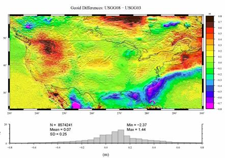
Figure 4 Differences between USGG2003 and USGG2009 mainly highlight the improvements to the underlying reference models. EGM96 was used for USGG2003, while EGM08 was used for USGG2009.
The changes from USGG2003 to USGG2009 are quite significant.
The long wavelength changes are due to the differences between the EGM96 and
EGM08, and the improved altimetric gravity anomalies. Over the oceans, there are
clear features that are associated with the mean ocean dynamic topography of
the
One final note on the USGG2009 model: it does not include any of the recently acquired airborne gravity data collected as a part of the Gravity for the Re-definition of the American vertical Datum (GRAV-D) project. This model is intended as a baseline for determining the impact of GRAV-D; see http://www.ngs.noaa.gov/GRAV-D/ for more details. As GRAV-D moves forward, updated gravimetric geoid models will reflect the improvements. Those models will be posted to the web under a separate location. As more data and improved techniques are applied, this series of models will eventually lead to the selection of the optimal gravimetric geoid for replacing the North American Vertical Datum of 1988.
4 GPSBM2009
Another essential data set for geoid modeling is the GPSBM’s derived from the differences between the NAD 83 and NAVD 88 datums on the bench marks. As GPS became operational in the early 1990’s, NGS quickly adopted the new technology and established High Accuracy Reference Networks (HARN’s) in each state. Ellipsoidal coordinates were readjusted then based on the other points in a state’s HARN through about 1998. At about that time, a nationwide network of Continuously Operating Reference Stations (CORS) was established.
This network provides not only the 3-D coordinates of stations, but also monitored the coordinates changes (velocities). HARN’s were now adjusted based on the CORS stations, to which new stations were constantly being added. This series of adjustments in conjunction with older baselines and other datum errors, led to the National Readjustment of 2007 (NRA2007). Prior to the NRA2007, approximately 18,000 points met the criteria for being used to make a hybrid geoid model. After that, the number dropped to closer 13,000. While the number of points used here represent approximately the same number as were available for GEOID03, the distribution and quality of these points has significantly changed.
The coordinate changes after NRA2007 directly impact the hybrid modeling, because the implied geoid heights are derived from the difference between NAVD 88 and NAD 83 on a bench mark – changing only the ellipsoid height on the bench mark creates a “new” geoid height. To a lesser extent, this has been the basis for rolling out new hybrid geoid models in the past. New models were published to reflect the current state of the database. It was necessary to hold off on publishing this model for this reason. We originally intended a GEOID06, but that became GEOID07, which became GEOID08, and finally became GEOID09. Holding off on this was necessary because of the magnitude of the changes. Certainly all coordinates changed, but the most important for geoid modeling is the ellipsoidal height change. Figure 5 shows the absolute changes in height.

Figure 5 Absolute height changes after the National Readjustment of 2007 (NRA2007). Note states like California with a highly noisy character and states like Minnesota with a significant trend.
The noticeable height changes happened in California, Alabama, Georgia, Minnesota and Alaska. The changes are a combination of the Earth’s dynamics (crustal motion, subsidence, glacial rebound) as well as the steady changes in coordinate adjustments (e.g., HARNS, CORS, NRA). Figure 5 highlighted the point differences, while Figure 6 shows their impact in the locales.
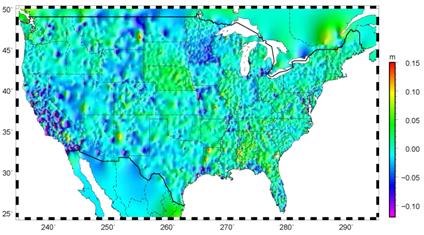
Figure 6 Height changes after the National Readjustment of 2007. Values are from Figure 5 and gridded to highlight regions where gaps in coverage create dm-level artifacts.
The GPSBM’s are relatively much sparser than the point gravity data by a couple orders of magnitude. Additionally, they tend to be clustered in states with active geodetic surveying programs. Hence, a given GPSBM control value may influence a large region around it. Gridding the data highlights the long wavelength artifacts that can result across gaps in the coverage. These gaps take the form of large features of significant (dm-level) magnitude and do not represent real signal. Hence, error estimates of hybrid geoid models are always overly optimistic as they assume a sufficiency of coverage throughout the country. Use of any hybrid geoid model should also rely on examining the coverage of the data used to make it.
Table 1. Comparisons between GPSBM2009 and USGG2009 & GEOID09. All values in cm. SD represents 1σ. Double that to get the 95% confidence level. The σh column represents the state average for all points for a given state derived from the NRA2007. AVE and SD are provided for both USGG2009 and GEOID09.
|
ST
|
No. Pts. |
σh cm |
USGG2009 |
GEOID09 |
|
ST |
No. Pts. |
σh cm |
USGG2009 |
GEOID09 |
||||
|
Ave. |
SD |
Ave. |
SD |
Ave. |
SD |
Ave. |
SD |
|||||||
|
AL |
53 |
1.3 |
-40.0 |
5.5 |
0.1 |
2.3 |
NE |
119 |
0.6 |
-75.8 |
4.4 |
-0.1 |
0.8 |
|
|
AZ |
153 |
0.8 |
-62.0 |
7.4 |
0.0 |
1.6 |
NV |
64 |
1.0 |
-82.8 |
8.0 |
0.1 |
1.4 |
|
|
AR |
58 |
1.2 |
-49.2 |
3.2 |
0.0 |
0.8 |
NH |
13 |
1.5 |
-41.6 |
2.9 |
-0.2 |
1.3 |
|
|
CA |
557 |
2.7 |
-83.2 |
12.2 |
0.0 |
2.3 |
NJ |
198 |
0.4 |
-42.9 |
2.7 |
0.0 |
1.1 |
|
|
CO |
459 |
1.1 |
-69.2 |
8.1 |
0.0 |
2.8 |
NM |
89 |
1.0 |
-51.3 |
8.9 |
0.0 |
1.4 |
|
|
CT |
8 |
1.7 |
-41.3 |
4.0 |
-0.1 |
1.6 |
NY |
105 |
1.2 |
-46.4 |
6.9 |
0.0 |
1.4 |
|
|
DE |
20 |
2.5 |
-40.3 |
4.2 |
0.2 |
2.5 |
NC |
1231 |
0.8 |
-35.8 |
5.2 |
0.0 |
1.7 |
|
|
DC |
16 |
0.6 |
-44.6 |
2.0 |
-0.2 |
2.0 |
ND |
41 |
0.7 |
-97.7 |
3.4 |
0.2 |
0.8 |
|
|
FL |
1413 |
1.6 |
-5.8 |
7.7 |
0.0 |
1.5 |
OH |
191 |
1.4 |
-60.4 |
5.0 |
0.0 |
2.0 |
|
|
GA |
95 |
1.2 |
-33.9 |
6.4 |
0.0 |
1.0 |
OK |
71 |
1.4 |
-51.8 |
5.4 |
0.0 |
1.0 |
|
|
ID |
87 |
1.4 |
-101.7 |
7.9 |
0.0 |
1.5 |
OR |
163 |
0.9 |
-108.7 |
8.5 |
0.0 |
1.4 |
|
|
IL |
266 |
1.1 |
-68.7 |
8.3 |
0.1 |
1.2 |
PA |
80 |
0.7 |
-49.8 |
4.1 |
0.0 |
1.1 |
|
|
IN |
113 |
1.1 |
-60.7 |
6.3 |
-0.1 |
2.0 |
RI |
15 |
0.9 |
-42.9 |
1.7 |
0.0 |
1.4 |
|
|
IA |
73 |
1.0 |
-77.4 |
4.9 |
0.0 |
0.8 |
SC |
663 |
1.0 |
-38.1 |
6.2 |
0.0 |
1.1 |
|
|
KS |
94 |
1.0 |
-65.9 |
5.3 |
0.0 |
1.2 |
SD |
172 |
1.1 |
-84.7 |
5.9 |
0.1 |
0.9 |
|
|
KY |
97 |
1.6 |
-50.2 |
4.1 |
-0.1 |
1.7 |
TN |
248 |
1.1 |
-49.9 |
3.7 |
0.0 |
1.9 |
|
|
LA |
343 |
1.0 |
-22.2 |
8.9 |
0.0 |
0.6 |
TX |
188 |
1.4 |
-36.8 |
8.1 |
0.0 |
2.4 |
|
|
ME |
57 |
0.9 |
-39.8 |
4.6 |
0.0 |
0.9 |
UT |
37 |
0.8 |
-79.8 |
9.1 |
0.1 |
2.1 |
|
|
MD |
186 |
0.8 |
-43.2 |
2.9 |
0.0 |
1.9 |
VT |
279 |
1.0 |
-42.1 |
4.3 |
0.0 |
1.3 |
|
|
MA |
30 |
1.1 |
-40.7 |
3.5 |
0.0 |
1.1 |
VA |
190 |
1.0 |
-41.6 |
4.5 |
0.0 |
1.8 |
|
|
MI |
199 |
2.0 |
-64.5 |
7.2 |
0.1 |
1.7 |
WA |
183 |
1.3 |
-116.4 |
8.2 |
0.0 |
1.9 |
|
|
MN |
2943 |
0.4 |
-87.3 |
3.6 |
0.0 |
1.0 |
WV |
41 |
1.2 |
-51.3 |
4.8 |
0.1 |
1.9 |
|
|
MS |
104 |
1.7 |
-44.8 |
4.3 |
0.0 |
1.6 |
WI |
551 |
0.3 |
-73.3 |
3.4 |
0.0 |
0.7 |
|
|
MO |
96 |
0.9 |
-58.7 |
5.3 |
0.0 |
1.1 |
WY |
89 |
2.2 |
-84.1 |
9.3 |
0.0 |
2.6 |
|
|
MT |
150 |
2.2 |
-101.3 |
8.7 |
0.0 |
1.7 |
all |
12961 |
1.2 |
-58.5 |
6.3 |
0.0 |
1.5 |
|
Table 1 shows the data that are available for the 2009 model. These data were cleaned in three steps. First, the error value determined from the NRA2007 was used as an initial filter. The data were broken up by state and a statewide standard deviation determined. Points that fell outside of two sigma (95% confidence level) were rejected. This process was repeated three times. This resulted in dropping 303 points. By performing this on a state-by-state basis, a relative parity was obtained by ensuring that those states with high quality data did not cause too many point to be unduly eliminated in states with poorer quality. Next, the points were compared to USGG2009 values interpolated to the bench mark locations. Raw differences were taken to see if any outliers existed. One was found at over 2 meters. Next, multi-matrix least squares collocation (MMLSC) was used in the initial development of GEOID09. In determining the statistical behavior of the model, two more points were found to lie outside the behavior of the others (double or more the residuals of any other points).
This is encouraging because it means that the use of the
ellipsoidal height error derived as a part of the NRA 2007 provides a real
diagnostic tool for locating problem bench marks. Note that 303 points were
located this way and only 3 others were found using techniques employed in the
development of GEOID03 and earlier models. The remaining 12,979 points with 579
added from
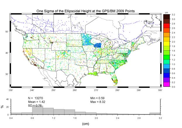
Figure 7 GPS-derived ellipsoid heights on leveled bench marks for 2009 (GPSBM2009). These point values represent the control data used to make GEOID09. The color scale shows the error estimate of the ellipsoidal height (σh) determined as a part of the NRA2007.
5 GEOID09
Finally, we get to the development of GEOID09. Most of the work has been completed in preparing the underlying gravimetric geoid, USGG2009, and cleaning the available GPSBM’s (GPSBM2009). The remaining task is to determine the best means of melding the two into a cohesive whole.
The general approach taken remains to determine the difference between and geoid height values determined by interpolating a gravimetric geoid (USGG2009) and the GPSBM’s (GPSBM2009). These residual signals mainly represent the misfit between the gravimetric geoid and NAVD 88. By developing a mathematical model from these control data, a conversion surface may determined to fit to the USGG2009 model that creates the GEOID09 model. The best tool for performing this fit was determined to be Multi-Matrix Least Squares Collocation (MMLSC) during the development of GEOID03 (Roman et al 2004). This tool was necessary due to the multiple complex features that correlated at different powers and scales of distance.
Before you can fit the model using MMLSC, any biases and trends must be removed. The trend for GEOID03 was 0.14 ppm, indicating that the mismatch between the NAVD 88 datum and the gravimetric geoid trended up 14 cm for every 1,000 km. For GEOID09, this number increased significantly to 0.31 ppm. This is largely due to the underlying reference model, EGM08, and is actually good news from a modeling perspective. First order trends are easy to model, it’s the features that span 10’s to 1000’s of km that are harder to model correctly. After removing the 0.14 ppm trend in 2003, the power of the remaining signal was (14.8 cm)2. In 2009, the power was reduced to (6.7 cm)2. With the bias and trend removed, MMLSC is employed to model this remaining signal.
Classical LSC permits fitting one Gaussian function that rolls off smoothly with distance. Unfortunately, the residual data implied here do not behave in this manner. MMLSC stacks multiple matrices to better emulate the actual data than the classical approach. Even though the magnitude of the signal to be modeled has been reduced, MMLSC was employed more extensively in 2009 to over come an earlier problem found in GEOID03.
GEOID99 (Smith and Roman 2001) used a single Gaussian function at 400 km. In 2003, only two functions were stacked: one at 60 km and the other at 650 km. This was later determined to be deficient in some regions where the data were much sparser than 60-120 km. In these regions, the only effective model was then at 650 km, which produced a poorer local comparison than for GEOID99. Most regions saw a drastic improvement under GEOID03 but not all.
Figure 8 Comparisons of analytic (MMLSC) models with empirical data for USGG2003 (left) and USGG2009 (right). Note that the scale for USGG2003 MMLSC is four times larger than for USGG2009. This indicates that there is less systematic signal to model. Also, note that the behavior of the curve is much smoother and fits better – indicating a better model.
Hence in 2009, six functions were stacked: 30 km, 60 km, 90 km, 120 km, 260 km, and 600 km. Figure 8 shows the comparisons between the math models and the empirical data for GEOID03 and GEOID09. Note that the left graph in Figure 8 has a scale on the Y-axis that is four times larger than the right figure due to the magnitude of the residual signal left after the trends were removed. The blue line shown in both plots represents the analytic signal derived from the math model (MMLSC). The black diamonds represent the binned values of the empirical data derived from the residuals between the gravimetric geoid and the GPSBM2009.
The analytic line in 2003 does a poorer job of fitting than
for 2009. This is because the character of the binned empirical data rolls off
more regularly in 2009 than in 2003. Note how the diamonds form a series of
humps in 2003. This is not so prominently the case in 2009. This is thought to
be because several state-sized features were removed from the residual signal
by cleaning up the GPS-derived ellipsoidal heights as a part of the NRA2007.
Recall that there was an obvious first order trend seen in Figures 5 and 6 in

Figure 9 Collocation surface determined for GEOID03 (left) and GEOID09 (right). Color scales are identical. Note difference in magnitude of modeled signal. Many features are gone or significantly reduced.
These are both at the same scale to highlight the magnitude
of the changes. Many features are no longer present. Examine in the left plot
the state of
These models were then added to trend surfaces derived from the 0.14 and 0.31 ppm trends determined for the respective models. Biases of around 58 cm were restored (common to both models), which likely represents the selection of Father Point/Rimouski as the datum point for NAVD 88. Also, a surface was added to account for the shift between NAD 83 and ITRF00 on which the USGG2009 and USGG2003 models are based. The conversion surface is then the sum of the collocation surface (from MMLSC), trend, bias, and ellipsoidal datum shift (ITRF => NAD 83). When the conversion surface is added to the gravimetric geoids, the hybrid geoids are determined. These models are then compared to the GPSM data again. No significant signal should remain as this whole effort has been to model these differences into the hybrid geoid models. Figure 10 shows the comparisons between GEOID03 (left) and GEOID09 (right) to their respective GPSBM data sets.

Figure 10 Comparisons of analytic (MMLSC) models with empirical data for GEOID03 (left) and GEOID09 (right). There is actually no signal to be seen in the right figure. The red dashed line shows the modeled residual values for GEOID03. GEOID09 is effectively precise to below a cm-level. The spikes on the Y-axes for both show the uncorrelated signal due to GPS random errors of observation.
What is remarkable here is that both did well. GEOID03 had around 1 cm of correlated signal that fell off quickly (10 km). Note where the analytic signal (blue line) intercepts the Y-axis – this value represents the correlated signal. The difference between this point and the spike on the Y-axis represents the uncorrelated signal (around (2.1 cm)2 in magnitude).
For GEOID09, this is even better. The red line is identical to the blue line shown in the left graph. This is necessary as there is no correlated signal remaining. Note how the empirical data (black diamonds) oscillate around zero almost up to auto-correlation, then there is a jump up to (1.5 cm)2 on the Y-axis.
In the Table 1, statistical values are given for all states
in CONUS and the
6 Other Regions
While other regions are not discussed here, it should be
noted that the scope of the models has been expanded. USGG2009 and GEOID09
models will be developed for
For
For the USVI in particular, a greater effort is being made. Their models will be out later this year and will reflect the likely first vertical datum based on a gravimetric geoid as a apart of the Gravity for the Redefinition of the American Vertical Datum (GRAV-D) project. High (35,000 ft) and low (5,000 ft) data will be combined with the existing data to create an improved gravimetric geoid model that will be used to define heights in the USVI. This exemplar will serve for how GRAV-D will be implemented eventually for the entire country.
Finally, DEFLEC09 models will be developed for all regions. These models will serve an expanding role in the GPS/INS community seeking continuity of navigation during times and places experiencing sporadic GNSS coverage.
7 Software and applications
The GEOID09 will be available on the NGS website through the Geoid web page and the NGS Geodetic Tool Kit:
http://www.ngs.noaa.gov/GEOID/
http://www.ngs.noaa.gov/TOOLS/
Descriptions and write-ups will be available on the respective pages in the Geoid respective web pages, while the data and tools to use it will be available through the Tool Kit.
8 Summary
USGG2009, GEOID09 and DEFLEC09 represent improved models for all users. USGG2009 incorporates the EGM08 reference field based on the GRACE data. It reflects improvements in terrain and processing and performs better than previous models. GEOID09 is based on this model and uses the most recent GPS-derived ellipsoidal heights on leveled bench marks (GPSBM’s) in the NGS database.
This is significant in view of the recent National Readjustment of 2007 that caused decimeters of change in ellipsoidal coordinates around the country. Use of earlier hybrid geoid models (e.g., GEOID03) will produce significant errors if used with the updated data available for NGS bench marks. Significant effort was made to ensure that GEOID09 better reflects the varying spatial distribution and quality of the GPSBM’s for each state. This effort has resulted in a hybrid model that will precisely provide the distance between NAD 83 and NAVD 88 based on the local spatial distribution. However, this does not address accuracy.
GRAV-D is being implemented in Puerto Rico and the U.S. Virgin Islands as a first step in defining a model that is both precise and accurate. The model will be available later this year and will be determined from dense, modern airborne gravity data.
Finally Deflection of the Vertical models (DEFLEC09) will be made available to assist in GPS/INS applications. These models will be developed for all regions as well.
Acknowledgments
Special thanks to Dr. Dru Smith for ideas and discussions centered on refining the Least Squares Collocation approach to better model local geoid height signals.
References
Anderson O.B., Knudsen P. (2008) Danish National Space Center 2008 Global Altimeter-Implied Gravity Anomalies (in press)
Barbarela, M., R. Barzaghi, D. Dominici, M. Fiani, S. Gandolfi, G. Sona: A comparison between Italgeo '95 and GPS/Levelling
data along the coasts of
Basic, T., M. Brkic, H. Sunkel: A new, more accurate geoid for
Behrend, D., H. Denker, W. Torge: Gravity field
determination in the German Bight (
Blitzkow, D., J.D. Fairhead, M.C. Lobianco: A
preliminary gravimetric geoid for
Blitzkow, D., M.C.B. Lobianco, J.D. Fairhead: Data
coverage improvement for geoid computation in
Clinton, William.
Denker, H.: Evaluation and
improvement of the EGG97 quasigeoid model for
Duquenne, H., M. Sarrailh: Improvement of gravimetric geoid determination in
the French Alps. Finnish Geodetic Institute Report 96:2, pp. 71‑76.
Proceedings, Session G7, EGS XXI Gen. Assembly,
Duquenne, H.: Comparison and combination of a gravimetric quasigeoid with a levelled GPS data set by statistical analysis. Phys. Chem. Earth (A), 24(1), 79‑83, 1999.
Duquenne, H.: QGF98, a new
solution for the quasigeoid in
Featherstone, W.E., J.D. Evans, J.G. Olliver: A Meissl‑modified Vanicek and Kleusberg kernel to reduce the truncation error in gravimetric geoid computations. Journal of Geodesy, 72(3), 154‑160, 1998.
Featherstone, W.E., M.G. Sideris:
Modified kernels in spectral geoid determination ‑ first results from
Forsberg, R., W. Featherstone.: Geoid and cap. In: R. Forsberg et al. (Eds.), Geodesy on the Move. IAG Symp. Proceed. vol. 119, pp. 18‑23, Springer, 1998.
Forsberg, R.: Geoid tailoring to GPS ‑ with examples
of a 1‑cm geoid of
Fukuda, Y., J. Kuroda, Y. Takabatake, J. Itoh, M. Murakami: Improvement of JGEOID93 by the geoidal heights derived from GPS/levelling
survey. In J. Segawa et al. (Eds.), Gravity, Geoid and Marine Geodesy IAG Symp. Proceed. vol. 117, pp. 589‑596, Springer, 1997.
Heiskanen, W. A., and H. Moritz, Physical Geodesy, W. H. Freeman and
Company,
Henning, W. E., E. E. Carlson, and D. B. Zilkoski, Baltimore County, Maryland, NAVD 88 GPS-derived Orthometric Height Project, Surv. Land Info. Sys., vol. 58, no. 2, pp. 97-113.
Ihde, J., U. Schirmer,
F. Toppe: Geoid modelling
without point masses. Finnish Geodetic Institute Report 98:4, pp. 199‑204.
Proceedings of the 2nd Continental Workshop on the Geoid in
Jiang, Z., G. Balmino,
H. Duquenne: On the
numerical approximation of the errors in a GPS aided gravimetric geoid
determination. Finnish Geodetic Institute Report 96:2, pp. 57‑66.
Proceedings, Session G7, EGS XXI Gen. Assembly,
Kenyeres, A.: A strategy for GPS heighting: the Hungarian solution. In J. Segawa et al. (Eds.), Gravity, Geoid and Marine Geodesy IAG Symp. Proceed. vol. 117, pp. 651‑658, Springer, 1997.
Koch, K.-R., Parameter Estimation and
Hypothesis Testing in Linear Models,
Kotsakis, C., M.G.
Sideris: On the adjustment of combined GPS/Levelling/Geoid networks. Presented at
the IV Hotine‑Marussi Symposium on Mathematical
Geodesy,
Milbert, D.G.: Improvements of a
high resolution geoid height model in the
Moritz, H., Advanced Physical Geodesy, Herbert Wichmann Verlag,
Ollikainen, M.: GPS levelling results obtained in
Pavlis NK, Holmes SA,
Roman, D. R., Y. M. Wang, W. Henning, J. Hamilton, Assessment of the New National Geoid Height Model—GEOID03, Surveying and Land Information Science, Vol. 64, No. 3, 2004, pp. 153-162.
Smith, D. A., and D. G. Milbert, The GEOID96 high resolution geoid height model for the United States, J. Geod., vol. 73, pp. 219-236, 2001.
Smith, D.A., and D.R. Roman, 2001, GEOID99 and G99SSS: One arc-minute models for the United States, J. Geodesy, vol. 75, pp. 469-490.
Wang, Y.-M., GSFC00 mean sea surface, gravity anomaly, and vertical gravity gradient from satellite altimeter data, J. Geophys. Res. Vol. 106 , No. C12 , p. 31167-31174, 2001.
Zilkoski, D. B., J. D. D'Onofrio, and S. J. Frakes,
Guidelines for