
| Other Laboratory Operations Food and Drug Administration |
| DOCUMENT NO.: III-04 | VERSION NO.:1.2 | Section 4 - Basic Statistics and Presentation | EFFECTIVE DATE: 10/01/2003 | REVISED: 06/27/2008 |
4.4 Linear Curve Fitting
This section deals with fitting of experimental data to a mathematical function.
This situation is encountered in a variety of situations in the ORA laboratory,
in particular with calibration curves. In most situations, the relationship
between the variables is linear, and therefore a linear function is needed:
y = f(x) = mx + b
Where x = independent variable,
y =
dependent variable,
m = calculated
slope of line, and
b = calculated
y-intercept of line.
The independent variable, x, is assumed to be known exactly,
with no error (such as concentration, distance, time, etc.). The dependent
variable, y, (instrument response for example) then depends
on (is a function of) the value of x. Each value of the independent
variable is assumed to follow a normal distribution and to have the same variance (i.e.
square of the standard deviation). The method of linear regression (also
known as linear least squares) is used to fit experimental data to a linear
function (note: in certain cases, a non-linear relationship may be reduced
to a linear equation by a transformation of variables; if so, the linear regression
method is still applicable).
The aim of linear regression is to find the line which minimizes the sum of
the squares of the deviations of individual points from that line. Once that
is accomplished, the slope (m) and the intercept (b) of the ‘least squares' line
is determined. It should be intuitively clear that minimizing deviations of
data points from the fitted line gives the best fit of data. Given a set of
data points (xi,yi), the equations used to determine the least squares
parameters are:


An additional parameter, which is an indicator of the "goodness of
fit" of the line to the data points, is the correlation coefficient. This
coefficient indicates how well the two data sets x and y correlate
with each other. The correlation coefficient, r2, uses information
on means and deviations of each data set to express this correlation numerically.
If the two data sets correspond perfectly, a correlation coefficient of 1 will
be calculated. A correlation coefficient of 0 indicates there is no relationship
between the two data sets. Typically, for analytical work performed in the
ORA laboratory, the correlation coefficient should be very close to 1 (for
example 0.999). The formula for the correlation coefficient is:

where terms have been defined previously.
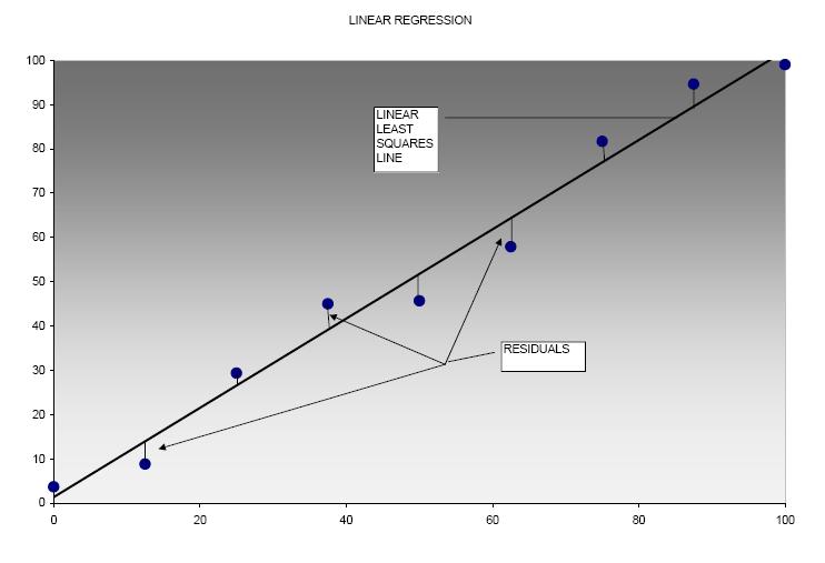
The following figure illustrates several points relating to linear least
squares curve fitting. Data was entered into an Excel® spreadsheet and
the linear least squares regression line calculated and plotted from the data.
The vertical lines indicate the distances (residuals) that are minimized
in order to achieve the best fit.
|


