|
July 19, 2005
The Risk Characterization component of the risk assessment is the integration of the Exposure Assessment and Dose-Response models. It provides estimates of the probability of illness and the overall annual illness burden attributed to consumption of oysters harboring pathogenic V. parahaemolyticus given current harvesting practices for each of the 24 region/season combinations. The influence of variability and uncertainty factors on the predicted risk were evaluated using statistical analyses. The risk assessment results were validated using data not included in the model.
Figure V-1 shows a schematic representation of all the parameters used in the simulation for each module and how the output of a module becomes an input for the following module. The probable numbers of illnesses were simulated separately for 24 region/season combinations. The predictions of illnesses were determined by the predicted distributions of the amount of pathogenic V. parahaemolyticus consumed and the dose-response relationship. Throughout the simulations, the uncertainty and variability was propagated through the various events along the pathway from harvest to consumption.
The calculations were performed by the Monte Carlo method of re-sampling from specified input distributions and appropriately combining the sampled values to generate the corresponding output distributions. In order to include the uncertainty and variability (as appropriate) for each model input, a total of 1,000 simulations were run for each region/season combination. Within each simulation there were 10,000 iterations which represent individual servings of raw oysters. Due to the relatively large number of servings consumed within each of the region/ season combinations, the numbers of illnesses were determined by multiplying the mean predicted risk per serving by the number of servings consumed. Additional details of the model are given in Appendix 3. A web address is also provided in Appendix 3, where a worksheet can be found which shows the different formulae, parameters and method of implementation of the Monte Carlo simulations.
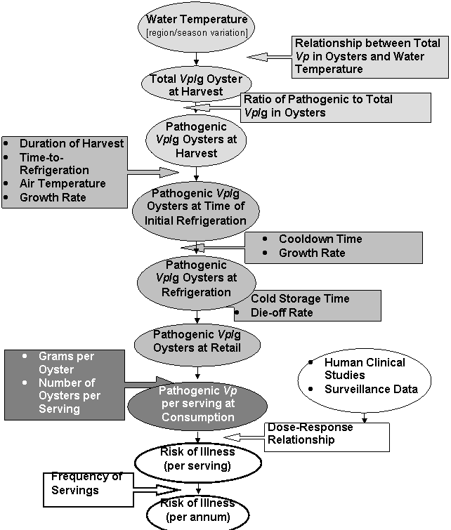
Figure V-1. Schematic Representation of the Vibrio parahaemolyticus Risk Assessment Model
[The light grey boxes with black lettering show the Harvest Module, the gray boxes with black lettering show the Post-Harvest Module, the dark grey boxes with white lettering show the Consumption Module, the white boxes with black lettering show the Dose-Response model, and the white boxes with dark black outline show the Risk Characterization.]
The "risk per serving" is the risk of an individual becoming ill (gastroenteritis alone or gastroenteritis followed by septicemia) when they consume a single serving of oysters. The predicted mean risk per serving for each region/season combination is shown in Table V-1. The predicted risk per serving is highest for the Gulf Coast (Louisiana) region and lowest for Pacific Northwest (dredged). Within a region, the risk per serving is highest for the warmer seasons (summer and spring) and lowest for the cooler seasons (fall and winter). For example, for the Northeast Atlantic, the risk per serving in the winter is approximately 1x10⁻⁸ meaning only one illness in every 100 million servings. For this same region, the risk per serving in the summer is approximately 3 orders of magnitude higher (one illness in every 100,000 servings).
The "risk per annum" is the predicted number of illnesses (gastroenteritis alone or gastroenteritis followed by septicemia) in the United States each year. The predicted mean risk per annum for each region/season combination is shown in Table V-2. The Gulf Coast accounts for approximately 92% (~2,600) of the predicted number of illnesses per year. The Gulf Coast (Louisiana) alone accounts for approximately 73% of predicted illnesses per year. The low numbers of illnesses predicted for the Northeast Atlantic and Mid-Atlantic oyster harvests are attributable to both the colder water temperatures and the relatively smaller harvest from these regions during the warm summer months.
The predicted number of cases of septicemia was determined for the total United States population as shown in Table V-3. The number of predicted cases of septicemia was estimated by multiplying the mean number of predicted illnesses (Table V-2) by the probability of gastroenteritis progressing to septicemia (0.0023). The derivation of the probability of gastroenteritis progressing to septicemia was described in Chapter III: Hazard Characterization (Table III-4). Most of the cases of illness are predicted to be associated with the Gulf Coast region oyster harvest and this is also the region associated with the highest number of cases of septicemia.
| Region | Mean Risk per Servinga | ||||
|---|---|---|---|---|---|
| Summer (July to September) | Fall (October to December) | Winter (January to March) | Spring (April to June) | Totalb | |
| Gulf Coast (Louisiana) | 4.4x10⁻⁴ (3.4x10⁻⁵, 1.4x10⁻³) |
4.3x10⁻⁵ (2.1x10⁻⁶, 1.5x10⁻⁴) |
2.1x10⁻⁶ (5.2x10⁻⁸, 8.3x10⁻⁶) |
1.7x10⁻⁴ (1.2x10⁻⁵, 5.4x10⁻⁴) |
6.6x10⁻⁴ |
| Gulf Coast (Non-Louisiana) c | 3.1x10⁻⁴ (2.3x10⁻⁵, 1.0x10⁻³) |
1.9x10⁻⁵ (7. 4x10⁻⁷, 6.6x10⁻⁵) |
1.1x10⁻⁶ (3.1x10⁻⁸, 4.2x10⁻⁶) |
1.2x10⁻⁴ (8.3x10⁻⁶, 3.9x10⁻⁴) |
4.5x10⁻⁴ |
| Mid-Atlantic | 9.2x10⁻⁵ (4.9x10⁻⁶, 3.3x10⁻⁴) |
2.2x10⁻⁶ (4.9x10⁻⁸, 1.0x10⁻⁵) |
1.1x10⁻⁸ (4.9x10⁻¹⁰, 3.8x10⁻⁸) |
3.1x10⁻⁵ (1.8x10⁻⁶, 1.1x10⁻⁴) |
1.3x10⁻⁴ |
| Northeast Atlantic | 1.8x10⁻⁵ (8.4x10⁻⁷, 6.9x10⁻⁵) |
4.0x10⁻⁷ (1.2x10⁻⁸, 1.6x10⁻⁶) |
1.1x10⁻⁸ (4.9x10⁻¹⁰, 3.5x10⁻⁸) |
3.6x10⁻⁶ (8.4x10⁻⁸, 1.5x10⁻⁵) |
2.2x10⁻⁵ |
| Pacific Northwest (Dredged)d | 1.0x10⁻⁵ (1.6x10⁻⁷, 4.2x10⁻⁵) |
2.6x10⁻⁸ (6.9x10⁻¹⁰, 9.5x10⁻⁸) |
8.1x10⁻¹⁰ (3.2x10⁻¹¹, 3.2x10⁻⁹) |
8.7x10⁻⁷ (4x10⁻⁹, 3.1x10⁻⁶) |
1.1x10⁻⁵ |
| Pacific Northwest (Intertidal)d | 1.4x10⁻⁴ (3.2x10⁻⁶, 6.2x10⁻⁴) |
3.9x10⁻⁷ (3.1x10⁻⁹, 1.6x10⁻⁶) |
1.7x10⁻⁹ (5.5x10⁻¹¹, 6.5x10⁻⁹) |
1.3x10⁻⁵ (2.3x10⁻⁸, 5.8x10⁻⁵) |
1.5x10⁻⁴ |
a Risk per serving refers to the predicted risk of an individual becoming ill (gastroenteritis alone or gastroenteritis followed by septicemia) when they consume a single serving of raw oysters. Values in parentheses are the 5th and 95th percentiles of the uncertainty distribution. Values rounded to 2 significant digits.
bNote: This value is the total mean predicted risk per serving, it is the rate of illness occurring of individuals who consume a single serving of oysters from the regional harvest in each of the four seasons.
c Includes oysters harvested from Florida, Mississippi, Texas, and Alabama. The time from harvest to refrigeration in these states is typically shorter than for Louisiana.
dOysters harvested using intertidal methods are typically exposed to higher temperature for longer times before refrigeration compared with dredged methods.
| Region | Mean Annual Number of Illnessesa | ||||
|---|---|---|---|---|---|
| Summer (July to Sept) | Fall (October to December) | Winter (January to March) | Spring (April to June) | Total | |
| Gulf Coast (Louisiana) | 1406 (109, 4435) | 132 (6, 468) | 7 (0.2, 26) | 505 (36, 1624) | 2,050 |
| Gulf Coast (Non-Louisiana)b | 299 (22, 985) | 51 (2, 180) | 3 (<0.1, 11) | 193 (13, 631) | 546 |
| Mid-Atlantic | 7 (0.36, 25) | 4 (<0.1, 17) | <0. 1 (<0.01, <0.1) | 4 (0.2, 15) | 15 |
| Northeast Atlantic | 14 (0.6, 53) | 2 (0.1, 7) | <0.1 (<0.01, <0.1) | 3 (<0.1, 12) | 19 |
| Pacific Northwest (Dredged) | 4 (<0.1, 16) | <0.1 (<0.01, <0.1) | <0.1 (0, <0.01) | 0.42 (<0.1, 2) | 4 |
| Pacific Northwest (Intertidal)c | 173 (4, 750) | 1 (0.01, 4) | <0.01 (<0.01, 0.01) | 18 (<0.1, 81) | 192 |
| TOTAL | 1,903 | 190 | 10 | 723 | 2826 |
a Mean annual number illnesses refers to predicted annual number of illnesses (gastroenteritis alone or gastroenteritis followed by septicemia) in the United States each year. Values in parentheses are the 5th and 95th percentiles of the uncertainty distribution. Note: Actual values for the illness predictions are provided in Appendix 7.
bIncludes oysters harvested from Florida, Mississippi, Texas, and Alabama. The typical time from harvest to refrigeration of oysters for these states is shorter than for Louisiana.
c Oysters harvested using intertidal methods are typically exposed to higher temperature for longer times before refrigeration compared with dredged methods.
| Region | Mean Annual Cases of Septicemiaa | ||||
|---|---|---|---|---|---|
| Summer (July to Sept) | Fall (October to December) | Winter (January to March) | Spring (April to June) | Total | |
| Gulf Coast (Louisiana) | 3 | <1 | <1 | 1 | 4 |
| Gulf Coast (Non-Louisiana)b | <1 | <1 | <1 | <1 | 1 |
| Mid-Atlantic | <1 | <1 | <1 | <1 | <1 |
| Northeast Atlantic | <1 | <1 | <1 | <1 | <1 |
| Pacific Northwest (Intertidal)c | <1 | <1 | <1 | <1 | <1 |
| Pacific Northwest (Dredged)c | <1 | <1 | <1 | <1 | <1 |
| TOTAL | 4 | <1 | <1 | 2 | 7 |
a Calculated by multiplying the estimated probability of septicemia (0.0023; Table III-4) by the mean predicted number of illnesses (Table V-2). Note: Actual values for septicemia cases shown as <1 are provided in Appendix 7.
b Includes oysters harvested from Florida, Mississippi, Texas, and Alabama. The typical time from harvest to refrigeration of oysters for these states is shorter than for Louisiana.
c Oysters harvested using intertidal methods are exposed to higher temperature for longer times before refrigeration compared with dredged methods.
The uncertainty of the predicted number of annual V. parahaemolyticus illnesses was analyzed for each region/season combination. The shape of the distribution is a consequence of model uncertainties based on 1,000 simulations. The predicted number of illnesses is greatly affected by the combination of the multiple uncertainties of all the inputs used in the model.
Figure V-2 provides an example uncertainty distribution for the Mid-Atlantic region for the spring and summer harvest seasons. The shape of the distribution is representative of each of the region/season combinations. In this example, 22% of the time (i.e., 220 of 1,000 simulations) the model predicted that approximately 8 illnesses each year were attributable to the Mid-Atlantic Summer harvest. Uncertainty distributions for the remaining region/season combinations are found in Appendix 8.
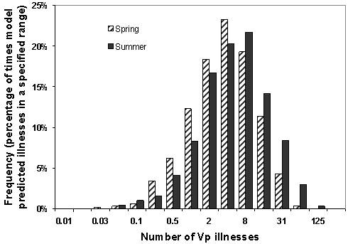
Figure V-2. Uncertainty Distribution of the Annual Number of Vibrio parahaemolyticus Illnesses Associated with Spring and Summer Mid-Atlantic Harvests
Statistical methods were applied to the model results for each region/season combination to identify and quantify the relative importance of both uncertainty and variability factors. These methods were applied to assess the importance of uncertainty and variability factors separately. Sensitivity analysis methods applicable to the context of food safety risk assessment models (Patil and Frey, 2004; Saltelli et al., 2000; Frey et al. 2004) were evaluated and the appropriate methods were selected for the analyses.
In this risk assessment, a distinction was made between model parameters that are uncertain versus those that represent "true" variability. As previously stated, within each of the 1,000 simulations of the model, there are 10,000 iterations which represent individual oyster servings. All values generated within an iteration of the model are variability factors. Uncertainties do not change within an iteration but do differ for each simulation. Two examples are provided below to illustrate the difference in variability and uncertainty as applied in the model.
The overall model was structured to separate variability and uncertainty factors to the maximum extent practical. The distinction between these two types of factors was maintained in sensitivity analyses of model simulation output because the principle effect of uncertainty is to shift the mean of the variability distributions of the predicted risk per serving. In contrast, variability factors affect the risk associated with individual servings as a consequence of V. parahaemolyticus levels varying from one harvest lot to the next, even when all uncertainty parameters are fixed.
A "segmented" approach was used for this risk assessment in that each of the 24 region/season combinations were simulated and analyzed separately. This approach was adopted as an effective means for specifying the diversity that exist in oyster harvesting practices and climatic conditions among the different regions. However, as a consequence of the segmented approach factors that affect risk have the potential to vary more strongly across different region/season combinations than within each region/season combination. This implies that evaluation of results for any particular region/season combination can not be inferred to apply directly to the aggregate of all 24 region/season categories.
Water temperature is the factor whose importance is most obscured by the segmented modeling approach. Within each region/season combination, the variation and impact of differing levels of water temperature is relatively minor in comparison to that of other model factors. However, this is not true across region/season categories. In fact, the wide variation of water temperature across different regions and seasons was one of the primary reasons for defining the various regions and seasons selected for the model. Across these region/season categories, changes in risk are strongly related to changes in water temperature as shown in Figure V-3.

Figure V-3. Influence of Water Temperature on Variation of Mean Risk per Serving for Each Region
A tornado plot is a convenient means of graphically depicting which factors in a model are the most influential. This type of plot is a graph of the correlations between the model output (i.e., risk) and various input factors (e.g., levels of V. parahaemolyticus in oysters at harvest). The graph is called a "tornado plot" because of the tornado-like appearance of the graph when factors are arrayed from most influential at the top to least influential at the bottom. It should be noted however, that factors with strong negative correlation are observed at the bottom of the plot, even though they may be more influential than a factor with a moderate positive correlation.
For this risk assessment, Pearson correlation between the model output and input factors was considered an appropriate correlation measure for the tornado plots. Although use of rank correlation is also applicable and potentially more robust than the Pearson correlation, care must be taken in interpretation of results obtained after rank transformation. The influence of factors which influence the output by way of interactions may not be appropriately identified when rank correlation is used (Saltelli and Sobol, 1995).
To ascertain the influence or importance of variability factors, Pearson correlations between the log risk/serving and selected inputs were calculated. Correlation against risk/serving is not appropriate because it is not normally distributed. Next, a mean correlation was obtained by taking the average over uncertainty samples. The tornado plots for each region/season combination are provided in Appendix 8. Several example graphs are provided below (Figures V-4 to V-7).
Table V-4 provides a summary of the tornado plot analyses of model variability factors. The most influential factor is the level of total V. parahaemolyticus in oysters at the time of harvest. It ranks highest for all region/seasons except for the Pacific Northwest winter harvests, where the ratio of pathogenic to total V. parahaemolyticus (% pathogenic) in oysters ranks highest. In general, the second most influential factor is the percentage pathogenic V. parahaemolyticus in oysters at harvest. Air temperature is another highly influential factor for most regions and seasons. It often ranks as the second most influential factor (see Table V-4 and Appendix 8). This is not surprising because the potential growth of V. parahaemolyticus in oysters during the time from harvest to refrigeration is a function of the ambient air temperature at the time of harvest and the length of time oysters are unrefrigerated. Vibrio parahaemolyticus will multiply in oysters until adequately chilled.
For the Pacific Northwest (Intertidal) harvest (Figures V-6 and V-7), the influence of oyster temperature and intertidal exposure time were also evaluated. For this region (and method of harvest) higher levels of risk per serving are associated with oysters that have been collected on warm sunny days leading to higher oyster temperatures and more V. parahaemolyticus growth during intertidal exposure. The lower rank of importance of the percentage of total V. parahaemolyticus that are pathogenic for this region and harvest type may be attributed to the relatively stronger influence of air (and oyster) temperature. The magnitude of the correlation of percentage pathogenic with risk per serving for this region is still comparable with that of the other regions such as the Gulf Coast or Mid-Atlantic. Intertidal exposure time is much less influential than other factors. This is attributable to the relatively narrow range of variation of this factor in comparison to that of other factors.
The other variability factors analyzed have significant effects, but to a lesser extent. In the Gulf Coast (Louisiana) and other "warm" regions, the time-to-refrigeration was generally the third most important influential factor affecting risk of illness. Serving size (number of oysters consumed) was another influential factor; the more oysters an individual consumes, the more likely it is that the person could become ill. Not surprisingly, conditions that foster the growth of V. parahaemolyticus within the oyster (length of time oysters are unrefrigerated, time it takes to cool down the oysters, water and air temperature) are all positively associated with the risk of illness. Since the levels of V. parahaemolyticus decrease during cold storage, the length of time the oysters are refrigerated is negatively correlated with the risk and that factor points the opposite direction on the tornado plot.
| Variability Factors in Order of Importancea | |||||||
|---|---|---|---|---|---|---|---|
| Season | Gulf Coast (Louisiana) | Gulf Coast (Non-Louisiana) | Mid-Atlantic | Northeast Atlantic | Pacific Northwest (Dredged) | Pacific Northwest (Intertidal) | |
| Summer |
|
|
|
|
|
|
|
| Fall |
|
|
|
|
|
|
|
| Winter |
|
|
|
|
|
|
|
| Spring |
|
|
|
|
|
|
|
aLog10 VP = log10 V. parahaemolyticus in oysters at harvest; % path= ratio of pathogenic to total V. parahaemolyticus in oysters at harvest; time unrefrig= time between harvest and refrigeration of oysters; air temp= ambient air temperature (used to determine oyster temperature after harvest); g consumed= grams of oysters consumed per serving; cooldown= time required for oyster to cool to no-growth temperature for V. parahaemolyticus; oyster temp= temperature of oysters during intertidal exposure; intertidal time= duration of time that intertidally-collected oysters are exposed prior to collection.
Note: Negatively correlated factors are not included in this table. For the actual tornado plots for each region/season combination see Appendix 8.
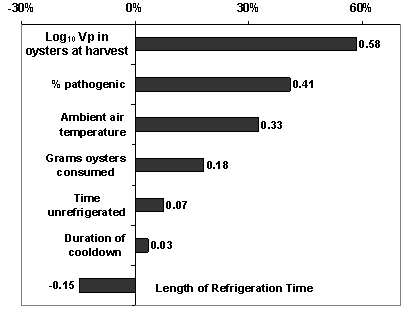
Figure V-4. Tornado Plot of Influential Variability Factors on Vibrio parahaemolyticus (Vp) Illness per Serving of Raw Oysters for the Gulf Coast (Louisiana) Winter Harvest
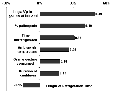
Figure V-5. Tornado Plot of Influential Variability Factors of Vibrio parahaemolyticus (Vp) Illness per Serving of Raw Oysters for the Gulf Coast (Louisiana) Summer Harvest
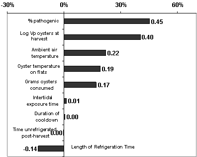
Figure V-6. Tornado Plot of Influential Variability Factors on Vibrio parahaemolyticus (Vp) Illness per Serving of Raw Oysters for the Pacific Northwest Coast (Intertidal) Spring Harvest
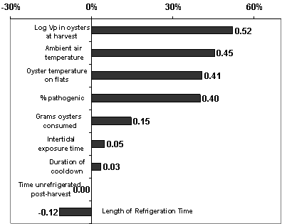
Figure V-7. Tornado Plot of Influential Variability Factors on Vibrio parahaemolyticus (Vp) Illness per Serving of Raw Oysters for the Pacific Northwest Coast (Intertidal) Winter Harvest
A potential deficiency associated with Tornado plots (i.e., pairwise correlations) as a sensitivity measure is that the importance of the factors is evaluated one at a time. Correlation between input factors themselves can confound the interpretation of importance in a Tornado plot. Therefore, to confirm and substantiate the results, a variance-based method of sensitivity analysis was also applied to two selected region/season combinations. The results of this analysis for the Gulf Coast (Louisiana)/Summer and Pacific Northwest (Intertidal)/Summer region/season combinations is given in Appendix 6. The results are generally consistent with the ranking of importance shown in Table V-4.
The correlation between predicted risk per serving and total V. parahaemolyticus density at the time of harvest for the Gulf Coast (Louisiana) summer harvest is shown in Figure V-8. While the correlation is high, indicating that V. parahaemolyticus levels at the time of harvest are an important indicator of risk, there is substantial variation (of risk) at any particular harvest level due to the influence of other factors. This illustrates that the usefulness of any indicator as a means to mitigate risk depends on the extent to which the factor can be controlled and this should be considered when assessing the value of identifying a factor with high influence. Additionally, it should be noted that this relatively high degree of importance in regard to indication of risk per serving does not necessarily equate with the most practical or economical avenues of mitigation. See "Chapter VI: What-If Scenarios" for information on the impact of various mitigation strategies on the predicted risk.
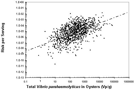
Figure V-8. Correlation of Risk per Serving and Total Vibrio parahaemolyticus in Oysters at Harvest for the Gulf Coast (Louisiana) Summer
[Individual simulation results are represented by a single dot. The dotted line is the least squares regression line fit to the simulation output.]
Simulations were performed to examine the influence of uncertainty factors on the predicted risk estimates. Five uncertainty factors were evaluated:
One measure of sensitivity (or importance) of these factors is the reduction in the variance of the uncertainty distribution of the mean risk per serving when each factor is held fixed to its nominal or mean level. If a factor has a substantial contribution to the overall uncertainty of the risk (i.e., is important), then there is a large reduction in the variance of the uncertainty distribution when the factor is held at a fixed level. This is most effectively summarized as the percentage reduction in the variance relative to that of the baseline uncertainty distribution of mean risk per serving (Saltelli et al., 2000). Thus, the importance (i.e., the percentage reduction in variance) is calculated according to the following formula.
| importance of the ith factor | = | Var(risk) - Var(risk | no variation of the ith factor) |
| Var(risk) |
where Var(risk) denotes the unconditional variance of the uncertainty distribution of mean risk per serving and Var(risk |no variation of the ith factor) denotes the conditional variance when one factor (the ith) is fixed.
As an example, this measure of importance was applied to rank the importance of the five selected uncertainty factors on predictions for the Gulf Coast (Louisiana)/Summer harvest. This region/season combination was selected because it represents the largest number of predicted illnesses. To estimate the conditional variances of the uncertainty distributions of mean risk per serving, 1,000 Monte Carlo simulations were performed for each of five model input factors. In each of these simulations, one of the five factors was fixed and the others were allowed to vary (as in the baseline model). The unconditional variance was also obtained based on a set of 1,000 Monte Carlo simulations in which all five factors were allowed to vary (as in the baseline model). The results of these simulations and the associated estimates of importance are summarized in Table V-5.
| Uncertainty Factor | Conditional Variancea | Importanceb |
|---|---|---|
| Dose-response model | 5.23x10⁻⁸ | 75.4% |
| Percentage pathogenic | 1.77x10⁻⁷ | 16.5% |
| Growth rate in oysters | 1.83x10⁻⁷ | 13.8% |
| Relationship of total V. parahaemolyticus levels and water temperature | 1.89x10⁻⁷ | 11.1% |
| Year-to-year water temperature variation | 2.08x10⁻⁷ | 2.0% |
a Conditional variance refers to the variance of the uncertainty distribution of the mean risk per serving conditional on the specified uncertainty factors being fixed to nominal (mean) values, one at a time.
b Importance is based on a comparison to an unconditional variance of 2.12×10⁻⁷ for the distribution of mean risk per serving from a simulation in which all uncertainty factors vary.
As shown in Table V-5, of the five uncertainty factors evaluated, the Beta-Poisson Dose-Response model ranks as the most important factor and has a substantial contribution (approximately 75% importance) to the uncertainty in the predicted mean risk per serving. The relative abundance of pathogenic strains in oysters and the growth rate of V. parahaemolyticus in oysters also contribute to the uncertainty in the results but to lesser degrees (i.e., approximately 14% and 16% importance each). The year-to-year variation of water temperature distributions ranks as the least important contributor to the uncertainty in the model results. In particular, the year-to-year variation in water temperature is extremely low. This reflects the fact that no appreciable year-to-year differences in Gulf Coast/Summer region water temperatures were evident in the NBDC data. This does not, however, necessarily imply that year-to-year variations of water temperature are equally inconsequential during other Gulf Coast seasons or in other regions. The importance of year-to-year variations of water temperature for other region/season combinations may vary somewhat, particularly for seasons during which the weather is more variable (e.g., spring and fall).
With respect to influence of dose-response uncertainty on the uncertainty of predicted mean risk per serving, it is worth noting, based on the model specification, that this is a reflection of parameter uncertainty of the Beta-Poisson model. Important sources of uncertainty that were not included in this assessment include those associated with the extrapolation of observed response at high doses to predicted response at low doses (i.e., model selection uncertainty). However, because a primary goal of the risk assessment was to evaluate the relative impact of different region/season combinations and to develop information on the impact of different intervention strategies, uncertainties associated with the dose-response model do not adversely impact the usefulness of the risk assessment.
An alternative method of importance assessment for these uncertainty parameters is to estimate the relative proportion of the variance of the uncertainty distribution of mean risk per serving explained by each uncertainty parameter in a regression-based approach (i.e., a "variance reduction" measure based on an approximating regression fit of model simulation output). The results of such an analysis (see Appendix 6) were found to be generally consistent with the ranking of importance as shown in Table V-5.
The model was evaluated by comparing model output predictions to similar data that were not used in the model. The exposure predictions were validated using data on the levels of total V. parahaemolyticus in oysters. Two evaluations were performed, one based on the ISSC/FDA retail survey and the other based on data collected by the Washington State Department of Health. These data were compared to model predictions to assess the appropriateness of the model with respect to the Harvest and Post-Harvest Modules.
Validation of the overall risk estimates requires detailed data on the number of illnesses associated with consumption of oysters harvested from the various regions and seasons. Such data are very limited and are, to an unknown degree, confounded. An attempt to evaluate the model in this manner was undertaken using data reported to the CDC on V. parahaemolyticus infections. These data were compared to the model's seasonal and regional predictions of illnesses. The number of V. parahaemolyticus cases predicted by the model was also compared qualitatively with preliminary data on the number of V. parahaemolyticus cases observed in the different provinces of Canada.
A collaborative survey of Vibrio parahaemolyticus densities in oysters at the retail level (i.e., restaurants, oyster bars, wholesalers) was conducted by the ISSC and FDA in 1998 and 1999 (FDA/ISSC, 2000; Cook et al., 2002a). Oyster samples were collected from selected states in the Pacific, Gulf Coast, Mid-Atlantic, and Northeast Atlantic regions. The samples were enumerated by an MPN method (Cook et al., 2002a). A relatively high proportion of the non-Gulf Coast samples had non-detectable levels. To adjust for the varying proportion of non-detectable V. parahaemolyticus across the different regions and seasons, estimated means were obtained by fitting a Tobit regression to the data with different harvest region and season combinations as a predictor variable. The variance about the group means was assumed to be the same across different regions and seasons, since no data were available to assume otherwise. The limit of detection varied somewhat from sample to sample but was generally 0.18 MPN/g.
Comparison of estimates of mean and standard deviation of log10 total V. parahaemolyticus densities from the ISSC/FDA study versus model predictions are shown in Figures V-9 through V-12 for the Gulf Coast (Louisiana), Gulf Coast (non-Louisiana), Mid-Atlantic, and Pacific Northwest (dredged and intertidal) regions. The data for the Northeast Atlantic region were not included in the analysis because the data set contained only few samples with detectable levels of V. parahaemolyticus. The estimates of the means based on ISSC/FDA data compare well with those predicted by the model. In particular, model predictions of mean log10 densities are in good agreement with ISSC/FDA data for all regions during the summer when the risk of illness is highest.

Figure V-9. Observed log10 Density of Total Vibrio parahaemolyticus at Retail (Cook et al., 2002a) Compared to Model Predictions for the Gulf Coast (Louisiana) Harvest [The error bars indicate one standard deviation above and below either the model predictions (square boxes) or observed values (filled circles).]
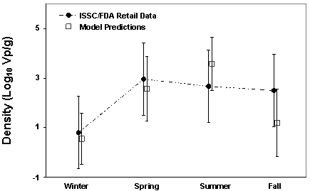
Figure V-10. Observed log10 Density of Total Vibrio parahaemolyticus at Retail (Cook et al., 2002a) Compared to Model Predictions for the Gulf Coast (non-Louisiana) Harvest [The error bars indicate one standard deviation above and below either the model predictions (square boxes) or observed values (filled circles).]
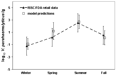
Figure V-11. Observed log10 Density of Total Vibrio parahaemolyticus at Retail (Cook et al., 2002a) Compared to Model Predictions for the Mid-Atlantic Coast Harvest [The error bars indicate one standard deviation above and below either the model predictions (square boxes) or observed values (filled triangles).]
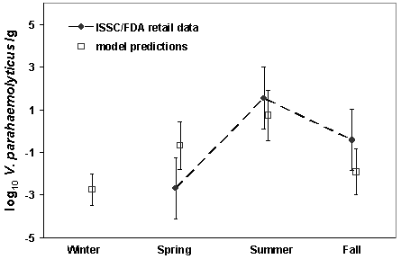
Figure V-12. Observed log10 Density of Total Vibrio parahaemolyticus at Retail (Cook et al., 2002a) Compared to Model Predictions for the Pacific Northwest (Dredged and Intertidal) Region [The error bars indicate one standard deviation above and below either the model predictions (square boxes) or observed values (filled circles).]
It should be noted that although the model predictions of the mean log10 densities vary from year to year based on environmental conditions; the ISSC/FDA data were collected from a single year. Therefore, differences in the model predictions and the ISSC/FDA estimates would be expected. For example, for the Gulf Coast (Figures V-9 and V-10), model predictions of mean log10 densities in the fall are somewhat lower than those obtained by the ISSC/FDA study. With regard to this discrepancy, water temperature measurements indicate that the fall season of 1998, corresponding to the time of ISSC/FDA sampling, was somewhat warmer than usual. Warmer temperatures allow more V. parahaemolyticus growth in oysters. The model was run to account for the higher temperatures for that year. Based on water temperature data from Weeks Bay, AL (NOAA, 2001), the mean daily water temperature in the fall of 1998 in the Gulf Coast region (Louisiana and non-Louisiana) was calculated to be 23°C (e.g., approximately 5°C warmer than typical fall mean daily water temperature of 17.8°C). As shown in Figure V-13, using the warmer water temperature data from 1998, the model predicts higher numbers of V. parahaemolyticus for the fall harvest and the values are similar to the ISSC/FDA retail study observed data. Therefore, this analysis, using a specific year's data, supports the validation and predictive capabilities of the model.
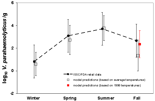
Figure V-13. Observed log10 Density of Total Vibrio parahaemolyticus at Retail
(Cook et al., 2002a) Compared to Model Predictions for the Gulf Coast (Lousisana and non-Lousisana) Based on 1998 Fall Temperature [The error bars indicate one standard deviation above and below either the model predictions using average temperatures (open square boxes) model prediction using only 1998 temperature data (filled square box) or observed values (filled circles).]
An additional validation was conducted for the Pacific Northwest (Intertidal) region using data collected from the intertidal areas of Hood Canal and South Puget Sound (Washington State Department of Health, 2001). This subset of the Washington State monitoring data was not used in the model. Comparison of the model predictions of intertidal "at-harvest" levels with the observed levels is shown in Figure V-14. The model-predicted mean log10 densities are similar to the regression-based estimate of the seasonal means. The results of a similar survey of V. parahaemolyticus levels in oysters harvested in the Vancouver area indicated a similar pattern as that observed in Washington State and predicted by the model (Buenaventura et al., 2004; Bannerjee and Farber, 2005).
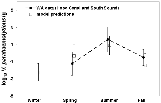
Figure V-14. Observed Log10 Density of Total Vibrio parahaemolyticus for the Pacific Northwest (Intertidal) Region (Washington State Department of Health, 2001) Compared to Model Predictions
[The error bars indicate one standard deviation above and below either the model predictions (square boxes) or observed values (filled circles).]
Based on the close agreement between model-predicted V. parahaemolyticus densities and observed densities at retail, the exposure assessment portion of the model is considered to be validated.
Surveillance data collected by CDC were compared to the model predictions in an attempt to validate the risk characterization portion of the model (also see Appendix 9). The comparison took into account the intrinsic difference in what the two systems (i.e., analysis of surveillance data versus model predictions) measure. The risk assessment model predicts illness associated with oysters harvested from a given region. Surveillance data, however, provide an estimate of illnesses reported within a region, regardless of the source of the oyster.
For reporting of a V. parahaemolyticus illness to appear in the CDC database, the following chain of events must occur:
There are several potential confounding factors with the CDC surveillance data which present difficulties in usig the surveillance data to validate the model predictions for harvest regions. First of all, CDC recognizes that there may be under diagnosing and underreporting of V. parahaemolyticus cases on a national basis. Therefore, the CDC includes an uncertainty factor of 20; the estimated total number of cases is equal to 20 times the reported cases (Mead et al., 1999). However, it is unknown the extent of possible differences in reporting efficiencies from state-to-state. Secondly, in only a small fraction (~10%) of the reported cases was it possible to definitively determine the source of the oysters that caused illness and attribute it to a particular region. There are also state-to-state differences in case follow up (traceback) procedures. These uncertainties associated with the surveillance data complicate the direct use of available CDC data to validate the regional model predictionns of illness.
The model predictions and the surveillance data estimates indicate similar trends in seasonal illnesses, with higher numbers associated with warmer months, fewer illnesses in cooler months, and the lowest number of illnesses in the winter. However, the model predictions of the number of V. parahaemolyticus illnesses in the winter were relatively low compared with the number of infections estimated from reported cases by the CDC. It is possible that the divergence between the CDC surveillance data and the predicted values reflect the existence of additional factors related to post-retail handling or consumption patterns of raw oysters during the winter months that have not been previously recognized and thus not incorporated into the model. Any consideration of such factors would require more sophisticated epidemiological investigations than those that are currently being performed. Alternatively, the differential could reflect the substantial uncertainty associated with the estimates derived from surveillance data.
As described above, the exposure assessment portion of the model is validated. However, the confounding factors and uncertainty associated with the surveillance data precluded validation of the risk characterization portion of the assessment. It is important to note that regardless of where the illnesses are reported and where the oysters were harvested, reducing exposure to Vibrio parahaemolyticus reduces the risk of illness. Various mitigations and control measures were evaluated and the effectiveness for different regions and seasons were determined as described in the next chapter, "What-If Scenarios." The validation of the exposure assessment provides a high degree of confidence that the impact of the various mitigation strategies considered would provide the risk reduction profile indicated in the "what-if" scenarios.