Estimating Link Travel Time Correlation: An Application of
Bayesian Smoothing Splines
BYRON J. GAJEWSKI1*
LAURENCE
R. RILETT2
ABSTRACT
The estimation and forecasting of travel times has become an
increasingly important topic as Advanced Traveler Information
Systems (ATIS) have moved from conceptualization to deployment. This
paper focuses on an important, but often neglected, component of
ATIS-the estimation of link travel time correlation. Natural cubic
splines are used to model the mean link travel time. Subsequently, a
Bayesian-based methodology is developed for estimating the posterior
distribution of the correlation of travel times between links along
a corridor. The approach is illustrated on a corridor in Houston,
Texas, that is instrumented with an Automatic Vehicle Identification
system.
KEYWORDS: Automatic vehicle identification, Gibbs Sampler, intelligent transportation systems, Markov Chain Monte Carlo.
INTRODUCTION
Estimating and forecasting link travel times has become an
increasingly important topic as Advanced Traveler Information
Systems have moved from conceptualization to deployment. Sen et al.
(1999) proposed estimating the correlation of travel times between
various links of a corridor as an open problem for future research.
In this paper, we assume that instrumented vehicles are detected at
discrete points in the traffic network, and links are defined as the
length of roadway between adjacent detection points. The set of
contiguous links forms a corridor. The link travel time for a given
instrumented vehicle is calculated based on the times at which each
of these vehicles passes a detection point.
Using these observations, link summary statistics, such as travel
time mean and variance as a function of time of day, can be
obtained. The travel time statistics for the corridor may be
obtained directly or be based on the sum of the individual link
travel times. In the latter case, a covariance matrix often is
required, because link travel times are rarely independent.
This paper focuses on estimating the correlation of link travel
times using Bayesian statistical inference. While the problem is
motivated and demonstrated using vehicles instrumented with
Automatic Vehicle Identification (AVI) tags, the methodologies
developed can be generalized to any probe vehicle technology. In
addition, while the AVI links have fixed lengths, the procedure can
be applied to links of any length.
The mean link travel time is a key input for estimating the
link-to-link travel time correlation coefficient. A continuous
estimate of the mean link travel time as a function of the time of
day is an important input to this process. In this paper, we use a
natural cubic splines (NCS) approach to estimate the mean travel
time as a function of time. The difference between each individual
vehicle travel time and the corresponding estimated mean travel time
is used, along with standard correlation equations, to obtain a
point estimate of the correlation coefficient. A technique for
calculating the variability of the estimate is also developed in
order to make inferences about the statistical significance of this
correlation coefficient.
Traditionally, variability is estimated using asymptotic theory.
However, for the travel time estimation problem, this approach is
complicated because of the nonparametric nature of the estimator and
the covariance between links. Consequently, we adopted a Bayesian
approach, which had a number of benefits in terms of interpretation
and ease of use. An added benefit to this approach is that the
actual distribution of the parameter is provided, which allows a
much broader range of statistical information, and consequently
better results, to be obtained. Further, we hypothesized that the
distribution of the correlation coefficient could be used by traffic
operations staff to help characterize the corridor in terms of the
consistency of individual vehicle travel times relative to the mean
travel time. As such, it may be considered a performance metric for
traffic operations.
In this paper, an 11.1 kilometer (km) (7.0 mile) test bed located
on U.S. 290 in Houston, Texas, was used to demonstrate the
procedure. AVI data were obtained from the morning peak traffic
period. We chose this time period because U.S. 290 experiences the
highest levels of congestion in the morning than at any other time,
and because estimating and forecasting travel times during congested
periods are considerably more complex than during noncongested
periods.
This paper is divided into four sections. First we present a
traditional approach to correlation coefficient estimation with a
special focus on the inherent complexities and difficulties. Next we
provide detailed discussion of the proposed Bayesian approach. The
third section demonstrates the methodology using AVI data observed
from the test bed and compares the Bayes approach to a more
traditional approach for estimating correlation. We found that the
estimates and their intervals can be calculated using the proposed
approach. Then, the estimated correlation coefficients are examined
from the viewpoint of traffic flow theory. The last section gives
concluding remarks.
We hypothesized that the positive correlation indicates the links
can be categorized as consistent in that drivers who wish to drive
faster (or slower) than the mean travel time can do so. Conversely,
if the correlation between links is negative, then the links can be
categorized as inconsistent. In this situation, drivers who are
slower (or faster) than average on one link are more likely to be
faster (or slower) than average on the other link. Finally, when the
correlation coefficient is at or near zero, then the system is
operating between the two extremes. Here, the drivers are unable to
maintain consistently lower or higher travel times between links,
again in relation to mean travel time, and the link travel times may
be considered independent. This latter case is often assumed in
corridor travel time forecasting and estimation, although the
assumption is rarely tested.
TRADITIONAL APPROACH AND SMOOTHING SPLINES
Over the last 10 years, most urban areas of North America have
seen extensive deployment of intelligent transportation system (ITS)
technologies. ITS traffic monitoring capabilites can be categorized
based on whether they provide point or space information. For
instance, inductance loop detectors provide point estimates of speed
and volume. Conversely, AVI systems provide space mean speed
estimates of instrumented vehicles. The focus of this paper is on
AVI-equipped systems. Note that even though the focus is on AVI
systems, the procedure can be readily generalized to other systems
that provide space information such as those that utilize global
positioning satellites or cell phone location technology.
Because of the nature of AVI systems, the speed of any one
vehicle at a given time is unknown; instead, the travel time (or
space mean speed) of each vehicle on each link is calculated based
on the time stamps recorded at each AVI reader. The travel time of
vehicle i along link l on any given day is defined as
Yil. Because the relationship between
travel time variability and time of day may be considered unstable,
a natural log transformation zil =
ln(Yil) is used to stabilize the
relationship. Assume that gil is the
expected value of zil. It is assumed that
the distribution of this transformation has a multivariate normal
(MVN) distribution as shown below:
![[lowercase z subscript {lowercase i lowercase l}] superscript {lowercase i lowercase i lowercase d} is approximately uppercase m uppercase v uppercase n ([lowercase g subscript {lowercase i lowercase l}, uppercase sigma]) for all lowercase i, lowercase l](https://webarchive.library.unt.edu/eot2008/20090512085008im_/http://www.bts.gov/publications/journal_of_transportation_and_statistics/volume_07_number_23/images/Gajewski-4.gif) (1) (1)
where
gil is a smooth function representing the mean
log travel time for link l; and
![uppercase sigma = [lowercase sigma subscript {lowercase l lowercase l suberscript {'}}], where [lowercase sigma subscript {lowercase l lowercase l subscript {'}] = lowercase sigma superscript {2} subscript {lowercase l} when lowercase l = lowercase l subscript {'}](https://webarchive.library.unt.edu/eot2008/20090512085008im_/http://www.bts.gov/publications/journal_of_transportation_and_statistics/volume_07_number_23/images/Gajewski-5.gif)
is the variance-covariance matrix of the log
travel time between links l and l′.
The normality assumption can be checked globally by inspecting
the residuals. In this paper gl , the
column vector of gil's from i =
1,...,n, will be estimated using NCS, an approach that is
discussed in detail elsewhere (Green and Silverman 1995; Eubank
1999). The fundamental calculation of an NCS is linear in nature.
For example,  , where zl is the column
vector of zil's, gives the mean log travel
time profile for a particular day on link l, where α
is the tuning parameter. The tuning parameter is discussed later,
and details for the calculation of A(α) are shown in
the appendix under "NCS Algorithm." , where zl is the column
vector of zil's, gives the mean log travel
time profile for a particular day on link l, where α
is the tuning parameter. The tuning parameter is discussed later,
and details for the calculation of A(α) are shown in
the appendix under "NCS Algorithm."
The test bed for this study is a three-lane section of U.S. 290
located in Houston. It has a barrier-separated high-occupancy
vehicle (HOV) lane that runs along the centerline of the freeway,
but the data utilized are from the non-HOV section of the freeway.
Eastbound (inbound) travel time data were collected over a 11.1
kilometer (7.0 mile) stretch of U.S. 290 from 4 AVI reader stations
(yielding 3 links). The lengths of links were 2.5 (1.6), 4.6 (2.9),
and 4.0 (2.5) kilometers (miles), respectively. The data were
collected over 20 weekdays in May 1996 from 6:00 a.m. to 8:00
a.m.
Figure
1 and table
1 outline an example of the above calculation for a subset of
the data (i.e., 18 observations on day 1 that begin at 7 seconds and
run to 6,822 seconds). In general, a tuning parameter, α,
that is too large produces a mean estimate that is too smooth and
does not follow the pattern laid out by the data. For example, it
can be seen that when α = 1x10¹¹, the NCS is
basically a decreasing straight line and captures none of the
traffic dynamics. Conversely, a tuning parameter that is too small
yields a rough NCS. It may be seen that when α =
8x10³, the function essentially runs through each
observation point and does not provide adequate smoothing. However,
for the intermediate value α = 3x10⁵, there is an
adequate tradeoff between the travel time dynamics and the
smoothing. Therefore, it is important to identify a tuning parameter
that is smooth but appropriately follows the dynamic trend. This can
be accomplished using visual inspection or by automatic
techniques.
A popular choice for automating the selection of the tuning
parameter is using the Generalized Cross Validation (GCV) method
(Green and Silverman 1995, p. 35). In this method, the smoothing
curve for one choice of tuning parameter is calculated without the
first value. Subsequently, the average square error is calculated
using the remaining values. This is repeated for all times during
the day. A modified version of the process eliminates the need to
remove each value by using the following formula:
 . .
In essence, a convex function of the tuning parameter is drawn
and the choice of tuning is the minimum of this function. The
advantage of using this procedure is that the process is
automated.
Figure
2 shows the log travel time as a function of time of day (6
a.m.-8 a.m.) for test bed links 1 and 2. For illustration purposes,
a subset of the vehicles has its log travel times highlighted with a
circle around the observation. In this particular example, the log
travel time experiences only slight changes during this period of
time: it begins relatively flat, experiences an increase at around
2,000 seconds and decreases starting at 4,000 seconds. Figure 2 also
shows three NCS where each one has a different tuning parameter. For
this example, a tuning parameter of α = 1x10⁵ was
chosen based on visual inspection and α =
0.065x10⁵ was identified based on the GCV process. For a
particular day, the same tuning parameter is applied to all links
along the corridor.
To illustrate the correlation between travel times on the two
links, consider the first highlighted vehicle that begins to
traverse link 1 at approximately t1 = 11 seconds.
Note that this vehicle has a lower than average travel time on both
links 1 and 2. The second highlighted vehicle begins to traverse
link 1 at approximately t = 548 seconds, and it can be seen
that its observed link travel times are above the mean travel time
on links 1 and 2. Eight of the 12 highlighted vehicles in figure 2
show evidence of positive correlation. Notice that this method
requires that the vehicles traverse both links, and vehicles
entering after the beginning of the first link or exiting before the
end of the second link are not included in the correlation
calculation. Later we employ these calculations for three links
where we include only vehicles that traverse the entire three-link
corridor.
To quantify the above relationship, we calculated the cross
product of the residuals. More specifically the covariance,
σ12 = E[ (zi1 −
zi1)(zi2 −
zi2) ] =
E[εi1 εi2]
and

where σ1 as defined earlier, was obtained using
the following procedure. The mathematical details of the procedure
are in the appendix under "Classic Estimation of Correlation."
Step 1: Transform the data to logarithms.
Step 2: Estimate the mean function by using NCS.
Step 3: Calculate residuals by subtracting the mean
function from the logarithm travel times.
Step 4: Estimate the variance and covariance using
the procedure outlined in the appendix.
Step 5: Calculate confidence intervals of the
correlation using standard asymptotic distribution theory (Wilks
1962).
For the example data shown in figure 2, the above procedure
resulted in an estimated correlation of  = 0.6918. This relatively high value reflects the
positive correlation for the log travel time of vehicles between the
links. = 0.6918. This relatively high value reflects the
positive correlation for the log travel time of vehicles between the
links.
Note that the above approach is problematic because it results
only in a partial solution. First, it would be desirable to have the
correlation coefficient for the untransformed data Y
il and not the natural log of the data, ln
(Y il ). Because the above correlation
coefficient reflects the transformed, rather than untransformed,
scale, interpretation is difficult. Secondly, and more importantly,
in order to make statistical inferences regarding the correlation
coefficient, the distribution of the untransformed correlation
coefficient is required. Identifying the distribution of the
untransformed correlation coefficient is equivalent to finding the
standard error of this estimate in the normal distribution case
using large sample theory. Additionally, because the correlation
calculation requires an estimate of the mean function using NCS,
this stage of uncertainty should be incorporated into the estimate
of the standard error. The entire process is very difficult to
accomplish, because the NCS and the sum of squares residuals need to
be calculated simultaneously. The traditional or classic approach
outlined in the appendix yields an approximation that does not
account for the uncertainty in the NCS. To overcome these
difficulties, an approach for obtaining the distribution of the
correlation coefficient on the untransformed scale using Bayesian
methodology is developed.
BAYESIAN APPROACH
To address the covariance problems identified in the preceding
section a Bayesian methodology is employed.
General Background
In Bayesian inference, the unknown parameters of the probability
distributions are modeled as having distributions of their own
(Gelman et al. 2000). Generally, the identification of the
distribution of the parameters, or prior distribution, is done
before the data are collected. Suppose that  is a vector containing unknown parameters with a
prior distribution is a vector containing unknown parameters with a
prior distribution  . The observed data are used to update this prior
distribution. The data are stored in the vector . The observed data are used to update this prior
distribution. The data are stored in the vector  and its distribution, conditional on the parameter
vector , is the likelihood and its distribution, conditional on the parameter
vector , is the likelihood  . The parameters' distribution is updated using the
Bayes theorem as shown below: . The parameters' distribution is updated using the
Bayes theorem as shown below:
 . (2)) . (2))
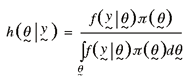
Once the posterior distribution, h(.,.), is identified, it
can be used to make inferences about the model parameters and to
identify the percentiles, the mean, and/or the standard deviation of
the distribution of the parameter.
Because the distribution shown in equation 2 is very difficult to
solve, a simulation method known as Gibbs Sampler or Markov Chain
Monte Carlo (MCMC) is used to approximate the distribution. This
approach has become increasingly popular over the last 10 years for
Bayesian inference (Gelfand 2002). The Gibbs Sampler is generally
constructed of univariate pieces of the posterior distribution. (For
more on the this topic, see the appendix under "Gibbs Sampler.")
Note that the Gibbs Sampler requires a number of simulation
replications that we denote as nreps.
The procedure is best illustrated by a simple example. Consider a
travel time/time-of-day relationship where the mean travel time does
not fluctuate and there is no need for an NCS (shown in figure
3). In this situation, it is reasonable to treat this
distribution as being normally distributed, yi ∼
N ( μ, σ2 ). In this case, the
parameter vector is

where µ is the mean travel time and σ2
is the variance of travel time. When choosing the prior
distributions, it is convenient to choose a distribution of a
conjugate form (Gelman et al. 2000). Because the posterior
distribution is of the same family as the prior distribution, it
leads to a straightforward complete conditional distribution. The
prior distributions of conjugate form that we adopted in this paper
are μ ∼ N(a, p2) and
σ2 ∼ IG(c,d), where IG
is the inverse gamma distribution. (A more detailed discussion of
the technical reasons for choosing conjugate prior distributions can
be found in Gelman et al. (2000). The details of the Gibbs Sampler
algorithm for the example are in the appendix under "Example Gibbs
Sampler.")
For the simple example, nreps was set to 2,000 and the
distributions are summarized with histograms as shown in figure 3.
In figure 3B, the mean parameter is summarized. The 5th and 95th
percentiles of  are 5.068 and 5.086 seconds, respectively. Because
of the simple nature of the example, it is possible to use standard
methods to calculate the 90% credible intervals. Note that the
classical t-distribution-based 90% confidence interval, which
would be 5.069 to 5.085 seconds, is comparable to the percentiles of
the Bayes approach because of the diffuse priors. An added advantage
of the simulation is that any function of the distribution can be
summarized. For example, figure 3C displays the distribution of
ln(σ2 ) in the form of a histogram. It
shows that, like the mean, the log variance tends to have a normal
distribution. This is similar to the normal distribution properties
associated with maximum likelihood estimators. are 5.068 and 5.086 seconds, respectively. Because
of the simple nature of the example, it is possible to use standard
methods to calculate the 90% credible intervals. Note that the
classical t-distribution-based 90% confidence interval, which
would be 5.069 to 5.085 seconds, is comparable to the percentiles of
the Bayes approach because of the diffuse priors. An added advantage
of the simulation is that any function of the distribution can be
summarized. For example, figure 3C displays the distribution of
ln(σ2 ) in the form of a histogram. It
shows that, like the mean, the log variance tends to have a normal
distribution. This is similar to the normal distribution properties
associated with maximum likelihood estimators.
Natural Cubic Spline Bayesian Method
While the idea of Bayesian NCS has been used in other
applications (Berry et al. 2002), here we expand the concept in
order to calculate the covariance function for the travel time for
vehicles between links. The travel time along link l when
starting at time ti is defined as
Yil. Because travel time variability is
unstable as a function of time, the variance is stabilized using a
natural log transformation zil =
ln(Yil). It is assumed that this
distribution will have a multivariate normal (MVN)
distribution with a smooth mean function and a fixed covariance
matrix as shown in equation 3 where:
[ zil ]iid ∼ MVN ( [
gil ], Σ
) ∀i,
l (3)
gl is a smooth function representing the mean
log travel time for link l; and

is the variance-covariance matrix of the log travel time.
This assumption can be checked globally in the model using Bayes
p-values (Gelman et al. 2000).
As discussed earlier, the area of focus is on the untransformed
space and, therefore, standard techniques are used to calculate
expectations of exponential space random variables (Graybill 1976).
The moment generating function (MGF) for the multivariate normal
distribution is m(t) = exp ( t′ μ +
t′ Σt / 2). Using this MGF, it can be shown that the
covariance for an individual vehicle between two links as a function
of time is
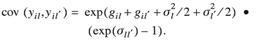 (4) (4)
The correlation coefficient of the untransformed data is shown in
equation (5), and it is important to note that it is not a function
of time. This allows a point estimate of the covariance between
links to be specifically obtained for any given day. This is shown
below:
 . (5) . (5)
The prior distribution of the smooth mean for link l
is
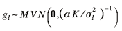
where K = α n Q B-1 Q′ and
α are used in calculating NCS and 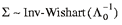 . The matrices Q and B are defined in
the appendix. "Inv-Wishart" denotes the inverse Wishart
distribution. If a non-informative version of the inverse Wishart
distribution is used, the following posterior distribution is
obtained: . The matrices Q and B are defined in
the appendix. "Inv-Wishart" denotes the inverse Wishart
distribution. If a non-informative version of the inverse Wishart
distribution is used, the following posterior distribution is
obtained:
 (6) (6)
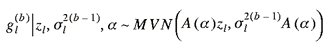
where
Σ | ε ∼ Inv-Winshartn(S)
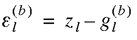
εl = zl −
gl, and

The above posterior distributions are extensions of the
multivariate calculations found in many Bayesian texts (e.g., see
Gelman et al. 2000). The distributions can readily be calculated
with a two-step Gibbs Sampler. The approach is summarized in the
appendix under "NCS Bayesian Algorithm."
The steps can be calculated easily in any matrix-based programs
that can simulate a multivariate normal distribution and an inverse
Wishart. For example, S-plus, MATLAB, R, or SAS-IML would be
appropriate.
DATA ANALYSIS
The methodology is illustrated on the test bed using three days'
data representing three different traffic conditions: moderate,
heavy, and light congestion. In all cases sampled, nreps is
set to 500.
An assessment of this log fit can be found using Bayes factors or
Bayes p-values (Gilks et al. 1996). In this paper, Bayes
p-values were used to verify model goodness-of-fit and to
check the validity of the underlying assumption. Two steps are
involved in this calculation. First, the predictive values of the
MCMC output are calculated using the MCMC model parameters. In this
paper, the predictive distribution for all links at
ti is
where
 and and
p stands for predictive distribution with the "b"th
iteration of the MCMC.
From the output, a χ2 discrepancy function is
calculated between the observed data and the parameters, as well as
between the predicted data and the parameters from the MCMC. The
discrepancy functions are calculated for each of the iterations of
the MCMC. In addition, the proportion of iterations from the MCMC
for which the data discrepancy is larger than the predicted
discrepancy is enumerated.
The flexibility in the choice of discrepancy function allows the
user to test many alternatives. The average within-link
auto-correlation per day is a relevant and interesting criterion to
test. This discrepancy function uses the standardized dataset's one
lag auto-correlation. The standardized data are

and the one lag correlation for the data and the predictive data
is
 and and
 . .
From this, the

A test using this choice of discrepancy function, on all days,
found that 75% of the days have a p-value within an
acceptable range of 0.01 to 0.99. The other 25% of the days report a
p-value less than 0.01. These latter p-values come
from days that have predominately free-flow traffic conditions.
These results indicate that while the model fits for traffic that is
dynamic, it needs additional work for free-flowing traffic days. It
is hypothesized that an extra parameter that accounts for
auto-correlation may reduce this discrepancy. Because free-flow
traffic conditions are not as interesting from a traffic monitoring
center (TMC) point of view, this extension is not performed here.
Figure
4 presents data for a day with moderate traffic congestion.
Figures 4A and 4B show the relationship between the log travel time
and time of day for links 1 and 2, respectively. In both instances,
the natural log travel time fluctuates between six (high) and four
(low). Using the Gibbs Sampler, the 5th and 95th percentile values
of the covariance of the travel times were calculated and are shown
in figure 4C. Note that the covariance is positive and fluctuates
proportionally to the mean travel times of the links. Because the
correlation result in equation 5 is time-independent, figure 4D can
be used to show the distribution of the correlation coefficient. The
distributions for the Bayes approach are summarized with the 5th and
95th percentile values. We refer here to this region as the 90%
Bayes credible region (BCR). The classic approach utilizes a 90%
confidence interval (CI) based on normal asymptotic theory. This
corresponds to a 90% BCR of (0.26, 0.42). The classic 90% CI was
slightly narrower (0.30, 0.45).
Figure
5 shows an analysis similar to that in figure 4 but for a day in
which the congestion is much greater. It can be seen that the
correlation is negative between adjacent links. The 90% BCR of the
correlation coefficient is (-0.39, -0.12). The classic 90% CI was
narrower and had a shift of (-0.42, -0.17).
Lastly, figure
6 shows a situation where the travel times are less dynamic with
high levels of free-flowing traffic, reflected by the positive
correlation. The 90% BCR of the correlation coefficient is (0.59,
0.69). The classic 90% CI is (0.61, 0.71). In summation, this
correlation coefficient reflects the amount of freedom an individual
vehicle has in traveling at a consistent speed relative to the
overall average travel time. Figure 6 shows a high positive
correlation, while figures 4 and 5 show correlation nearer zero or
negative correlation, respectively.
The "C" component of all three figures reports the covariance as
a continuous function of the time of day (equation (4)). It is the
pretransformed space that allows for interpretations on the original
scale. Notice that the fluctuations are proportional to the mean
travel time from the NCS. This result illustrates the distinct
advantage of the Bayes approach over the frequentist approach. In
order to derive a confidence interval when using a frequentist
approach, a large sample size is required to be able to apply the
linear assumption used in asymptotic theory. In addition, there is a
propagation of the uncertainty in the covariance because there are
several steps in its estimation. For example, there is a logarithm
transformation and an adjustment for the smooth mean via NCS.
In contrast, the Bayesian approach does not rely on the large
sample size assumption. In addition, the nature of the MCMC
iterations implicitly accounts for the transformed space.
Specifically, the covariance function's actual distribution is
calculated while ensuring that all forms of error are propagated.
However, given the large number of probe vehicles observed, it seems
conceivable that the large sample properties hold. Therefore, we
compare the frequentist-based approach (or classic approach) to the
Bayesian method.
One interesting result is that for any given day equation (5)
summarizes the correlation between pairs of links. Because the
equation relies on the variance and covariance between links, which
requires the estimate of the mean travel times, the distribution
still needs a method that includes the error propagation mentioned
above.
Figure
7 summarizes the correlation coefficients for all 20 days. The
correlation BCR percentiles for all three links and their pairs are
shown along with the classic 90% CI that appears next to the BCR for
comparison purposes. For the adjacent links 1 and 2, there are four
days that either have a negative correlation or a correlation where
the 90% BCR covers zero. There are six such days between the
adjacent links 2 and 3. The results are consistent for the
non-adjacent links (i.e., links 1 and 3). This illustrates that the
nonpositive correlation remains constant from link to link and seems
to be a within-day characteristic.
Also, in terms of space mean speed, this correlation measure can
be compared with traditional traffic congestion measures. Suppose a
link is considered congested when the speed falls below 56 km/hr (35
mph). For the first 12 days, all links had a minimum space mean
speed that ranged from 8 km/hr (5 mph) to 32 km/hr (20 mph). This
latter case corresponds to days when the 90% BCR was below 0.5. In
contrast, the last eight days have a minimum space mean speed
ranging from 73 km/hr (45 mph) to 105 km/hr (65 mph) and at least
one link pair with a 90% BCR covering 0.5. This demonstrates that
the single correlation measure matches traditional measures of
congestion that are based on speed. In general, the heavier the
congestion, the lower the correlation of travel time between
links.
Indeed, an obvious question raised by figure 7 is to ask whether
the MCMC method is necessary or if the classic approach is an
adequate approximation. The lengths of their respective 90%
intervals indicate that on average the Bayes intervals are 10.5%
longer than the classic intervals. The MCMC approach has longer
intervals because it accounts for the uncertainty in the estimate of
the smoothing spline. The user of our algorithm may want to balance
the gain in the MCMC approach with the loss in time it takes to
implement the algorithm. For the data from day 1, the 500 MCMC
iterations take 36 seconds to implement using MATLAB on a 2.00 GHz
processor with 1.00 GB RAM, whereas the classic approach takes less
than 1 second to implement. This difference in implementation time
might be different but is well worth the effort for those users who
wish to account for all of the uncertainty generated in the estimate
of interlink correlation. Given the rapid increase in computational
abilities, it is our belief that computation concerns will not be a
deciding factor.
The NCS smoothing technique is commonly used in statistics but
not extensively in transportation engineering. There is an explicit
tradeoff between the tuning parameter and the fitted curve, and it
is important that the tuning parameter be selected in an appropriate
and consistent manner. Figure
8A shows the correlation between links 1 and 2 (i.e.,  ) as a function of the logarithm of the tuning
parameter value for day 7. The arrow represents the "optimal" tuning
parameter based on the Generalized Cross Validation method. However,
note that in that figure (8A), the sign of the correlation is
positive for tuning values but negative for others. Therefore, it is
important that the tuning parameter be identified correctly,
otherwise the correlation value might be not only erroneous but of a
different sign. ) as a function of the logarithm of the tuning
parameter value for day 7. The arrow represents the "optimal" tuning
parameter based on the Generalized Cross Validation method. However,
note that in that figure (8A), the sign of the correlation is
positive for tuning values but negative for others. Therefore, it is
important that the tuning parameter be identified correctly,
otherwise the correlation value might be not only erroneous but of a
different sign.
Figures
8B and 8C
show the correlation between links 1 and 2 (i.e., ) as a function of the logarithm of the tuning
parameter value for days 10 and 20, respectively. The link-to-link
correlation seen in these figures is relatively high and stable. For
these examples, the travel time fluctuation is relatively smooth,
and the large values of the tuning parameter safeguard the dynamic
trend.
CONCLUDING REMARKS
This paper demonstrates that for the travel time estimation
problem the traditional approach is complicated because of the
nonparametric nature of the estimator and the covariance between
links. We adopted a Bayesian approach that had a number of benefits
in terms of interpretation and ease of use. As an added benefit,
this approach provided the actual distribution of the parameter,
which allowed a much broader range of statistical information, and
consequently better results, to be obtained. We found that, contrary
to a common assumption used in many transportation engineering
applications, the link covariance is non-zero. Furthermore, the
distribution of the correlation coefficient has the potential to be
used as a performance metric for traffic operations.
From a transportation engineering perspective, this work is
important for two reasons. First, this paper shows that the common
assumption that link travel time covariance is zero is erroneous.
More importantly, we developed a method for calculating the
covariance with appropriate intervals. This technique can be readily
incorporated for calculating travel time variance and the associated
interval. This will have relevance in a wide range of applications
including route guidance and traffic system performance measurement.
Secondly, correlation coefficients have the potential for
categorizing the performance of the traffic system, because they are
a direct measure of how constrained drivers are with respect to
traveling at their desired speed. The use of the proposed technique
in the above transportation applications will be the focus of the
next step in the research.
Two caveats to our study are as follows. First, the results
depend on the length of the links in which the vehicles traverse.
Suppose that the travel times for the three links have a positive
correlation. However, if for that distance the links were shorter
(i.e., six links over the same length) there is no guarantee the
relationship will remain the same (e.g., all six links are
positively correlated). No study finds the extent to which this
occurs. This issue could be addressed in future research by
utilizing a vehicle simulation program such as TRANSIMS (2003). With
this simulation program, the researcher can examine these types of
issues by playing "what if" scenarios with variations of the length
of the links under assorted dynamic and complex traffic conditions.
The second caveat to our study is that during severely congested
traffic, link travel times are essentially constant. In this case,
researchers will find it difficult to utilize link travel time
correlation as a congestion measure. This case is similar to the
free- flow case where drivers can go at the speed they wish. In both
situations, sophisticated congestion measures are not needed.
However, when things are rapidly changing, this approach would be
very useful. We show that the method is appropriate under several
dynamic conditions, where the speed ranged from 8 km/hr (5 mph) to
105 km/hr (65 mph). These would be the most interesting traffic
conditions (e.g., where the travel time fluctuates in and out of
free-flow and congested traffic conditions) from a traffic
management perspective.
ACKNOWLEDGMENTS
This research was funded in part by the Texas Department of
Transportation through the TransLink® Research Center. The
TransLink® partnership consists of the Texas Transportation
Institute, Rockwell International, the U.S. Department of
Transportation, the Texas Department of Transportation, the
Metropolitan Transit Authority of Harris County, and SBC Technology
Resources. The support of these organizations, as well as other
members and contributors, is gratefully acknowledged. We thank two
referees and the editor for helpful and insightful reviews that
greatly improved this article. The authors would also like to thank
Mary Benson Gajewski and Beverley Rilett for editorial assistance in
the preparation of this article.
REFERENCES
Berry, S.M., R.J. Carrol, and D. Ruppert. 2002.
Bayesian Smoothing and Regression Splines for Measurement Error
Problems. Journal of the American Statistical Association
97(45):160-169.
Eubank, R.L. 1999. Nonparametric Regression and
Spline Smoothing, 2nd edition. New York, NY: Marcel Dekker.
Gelfand, A.E. 2002. Gibbs Sampling. Statistics in
the 21st Century, Edited by A.E. Raftery, M.A. Tanner, and M.T.
Wells. Chapman & Hall and American Statistical Association,
Washington, DC.
Gelman, A., J.B. Carlin, H.S. Stern, and D.B. Rubin.
2000. Bayesian Data Analysis. London, England: Chapman &
Hall.
Gilks, W.R., S. Richardson, and D.J. Spiegelhalter.
1996. Markov Chain Monte Carlo in Practice. London, England:
Chapman & Hall.
Graybill, F.A. 1976. Theory and Application of the
Linear Model. Belmont, CA: Wadsworth.
Green, P.J. and B.W. Silverman. 1995. Nonparametric
Regression and Generalized Linear Models. London, England:
Chapman & Hall.
Ruppert, D., M.P. Wand, and R.J. Carroll. 2003.
Semiparametric Regression. Cambridge, England: Cambridge
University Press.
Sen, A., P. Thakuriah, X.Q. Zhu, and A. Karr. 1999.
Variances of Link Travel Time Estimates: Implications for Optimal
Routes. International Transactions in Operational Research,
(6)75-87.
TRANSIMS. 2003. Available at http://transims.tsasa.lanl.gov/,
as of May 2004.
Wilks, S.S. 1962. Mathematical Statistics. New
York, NY: Wiley.
APPENDIX
NCS Algorithm
The travel times for each of the individual vehicles are
yl1, yl2,
yl3,..., yln and
are recorded at times t1,...,
tn. The steps for calculating
A(α)are as follows:
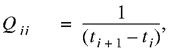
1. Let Q be a matrix of zeros of dimension n-2 by
n. For i from 1 to n-2 let


2. Let B be a matrix of zeros of dimension n - 2 by
n- 2.
For i from 2 to n - 3 let Bii -
1 = ti+ 1 - t
i,
Bii =
2(ti+2 -
ti ) and
Bii+1 =
ti+2 -
ti+1.
Let B11 = t2-t1,
B12 = t3-t2,
Bn-2n-3 =
tn-1-tn-2 and
Bn-2n-2=
tn-tn-1.
3. Set
B = B/6.
4. A (α) = In - n α Q′
(n α Q Q′ + B )-1 Q.
5. The quantity being analyzed is A (α)
zl, where zil =
log(yil).
Classic Estimation of Correlation
The correlation between two links,
![lowercase sigma caret subscript {1 2} = uppercase e [(lowercase z subscript {lowercase i 1} - lowercase g subscript {lowercase i 1})(lowercase z subscript {lowercase i 2} - lowercase g subscript {lowercase i 2})] = uppercase e [lowercase epsilon subscript {lowercase i 1} lowercase epsilon subscript {lowercase i 2}]](https://webarchive.library.unt.edu/eot2008/20090512085008im_/http://www.bts.gov/publications/journal_of_transportation_and_statistics/volume_07_number_23/images/Gajewski-76.gif) , ,
is estimated using the following procedure:
1. Given the tuning parameter α, use an NCS to derive a
continuous estimate of the mean travel time over the analysis period
for the two links and call them  and and  . .
2. For each link estimate the residuals for each vehicle:  and and  . .
3. Calculate the equivalent degrees of freedom (EDF):

4. Estimate the covariance between links 1 and 2:
 . .
Estimate the variance for links 1 and 2 respectively:
 . .
5. Calculate the estimated correlation:

Note that the basic concept of EDF is to penalize the
estimation of the covariance matrix using the proper equivalent of
degrees of freedom. The EDF for splines is discussed in Green
and Silverman (1995) and Ruppert et al. (2003).
Inferences utilizing the above approach can be accomplished with
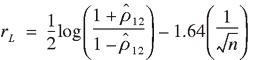
large sample distribution theory based on Wilks (1962, p. 594). The
result indicates that as the number of vehicles approaches infinity
the statistic ![1/2 log [(1 + lowercase rho caret subscript {1 2}) / (1 - lowercase rho caret subscript {1 2})]](https://webarchive.library.unt.edu/eot2008/20090512085008im_/http://www.bts.gov/publications/journal_of_transportation_and_statistics/volume_07_number_23/images/Gajewski-86.gif) has an approximate normal distribution with mean
and variance 1/n . Thus, this distribution is
used to calculate a 90% confidence interval with the formula has an approximate normal distribution with mean
and variance 1/n . Thus, this distribution is
used to calculate a 90% confidence interval with the formula
![[(exp (2 lowercase r subscript {uppercase l}) - 1) divided by (1 + exp (2 lowercase r subscript {uppercase l})) , (exp (2 lowercase r subscript {uppercase u}) - 1) divided by (1 + exp (2 lowercase r subscript {uppercase u))]](https://webarchive.library.unt.edu/eot2008/20090512085008im_/http://www.bts.gov/publications/journal_of_transportation_and_statistics/volume_07_number_23/images/Gajewski-88.gif)
where
 and and
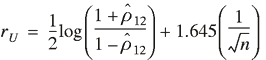 . .
The 1.645 corresponds to the 90th percentile of the standard
normal.
Gibbs Sampler
The approach is simulation-based where nreps is the number
of simulations performed on the parameter vector and b =
1,2,3,...,nreps. The Gibbs Sampler begins with a reasonable
starting value  (i.e., estimates of the parameters from a
traditional approach). From this starting value, the
kth component of is updated conditional on the data and all the other
components of the parameter vector, (i.e., estimates of the parameters from a
traditional approach). From this starting value, the
kth component of is updated conditional on the data and all the other
components of the parameter vector, 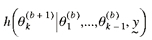 . The next step is to simulate the subsequent
component of the parameter vector . The next step is to simulate the subsequent
component of the parameter vector 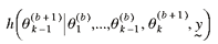 . This is repeated for all unknown parameters until
nreps simulations for each component of the parameter vector
have been completed. . This is repeated for all unknown parameters until
nreps simulations for each component of the parameter vector
have been completed.
Example Gibbs Sampler
The following steps are used to perform the Gibbs Sampler
simulation:
1. Set the prior distribution parameters to be diffuse
a = 0, p2 = ∞, c = 0 and
d = 0.
2. Set the starting values for the unknown parameters
 . .
3. Generate the mean portion
 , ,
which is of conjugate form (see Gelman et al.
2000 for the derivation).
4. Generate the variance portion
 , which is of conjugate form. , which is of conjugate form.
5. Repeat steps 3 and 4 nreps times.
NCS Bayesian Algorithm
For convenience, the approach is summarized in algorithmic
form:
1. Calculate zil =
ln(Yil).
2. Obtain the starting values  and Σ(1) using techniques previously
discussed in the section, "Traditional Approach and Smoothing
Splines." and Σ(1) using techniques previously
discussed in the section, "Traditional Approach and Smoothing
Splines."
3. Simulate
 . .
Note that the same tuning parameter will be used throughout the
algorithm. The g's and Σ are defined in equation (3).
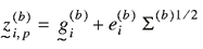
4. Calculate
Σ b+1 | ε(b) ∼
Inv-Winshartn(S(b)),
where
 and and 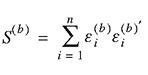 . .
5. Summarize the function(s) of the unknown parameters.
ADDRESSES FOR CORRESPONDENCE
1 Corresponding author: B.
Gajewski, Assistant Professor, Schools of Allied Health and Nursing,
Biostatistician, Center for Biostatistics and Bioinformatics, Mail
Stop 4043, The University of Kansas Medical Center, 3901 Rainbow
Blvd., Kansas City, KS 66160. E-mail: bgajewski@kumc.edu
2 L. Rilett, Keith W. Klaasmeyer Chair in Engineering and Technology and Director Mid-America Transportation Center, University of Nebraska-Lincoln, W339 Nebraska Hall, P.O. Box 88053, Lincoln, NE 68588-0531. E-mail: lrilett@unl.edu
|