Measurement Errors in Poisson Regressions: A Simulation Study Based on Travel Frequency Data
ERLING HÄGGSTRÖM LUNDEVALLER *
ABSTRACT
This paper considers how measurement errors in explanatory variables affect the analysis of a Poisson regression model for frequencies of recreational and shopping trips. Measurement errors can introduce bias into the parameter estimates, and the effects on this particular dataset and model are investigated. The structure of the data, with two observations for each individual, makes it desirable to test for correlation within each individual. It is possible that tests of random effects are sensitive to measurement error. The properties of tests of random individual effects when there are measurement errors are therefore studied in the paper. The results of a simulation study show that classical measurement errors cause severe bias, and Berkson measurement errors produce little bias. The tests for random individual effects work well both with measurement error and negatively correlated responses according to the simulation study.
KEYWORDS: Poisson regression, measurement error, travel frequencies, random coefficients.
INTRODUCTION
An often encountered situation in statistical modeling in various research fields is when the response variable of interest consists of frequencies. A widely used model for frequency data is the Poisson regression model. This modeling approach makes it possible to relate the response counts to explanatory variables. Although other models for frequency data can also be used, the Poisson model is in many cases the preferred model.
The quality of the data is of central importance for the results of the statistical analysis. One common problem is measurement errors in regressors. It is well known that measurement errors in explanatory variables introduce bias and inconsistency in estimators in linear regression models (e.g., Fuller 1987; Carrol et al. 1995). In a simulation study, Zidek et al. (1996) consider the Poisson regression model and present results indicating additional inconsistency problems under the combination of measurement errors and multicollinearity. Their research suggests potential problems with the validity of the results obtained in studies based on applications of the Poisson regression model.
In this paper, a travel frequency model (e.g., Hausman et al. 1995) assuming a Poisson distribution with potential measurement errors is studied. The data used contain information about the number of recreational and shopping (purchase) trips made by respondents. Recreational trips are made for leisure activities, while purchase trips are made for acquiring goods or services. One topic addressed here is the degree of bias introduced in the estimates of the Poisson regression model when explanatory variables are measured with error. The results presented in this paper add to those of Zidek et al. (1996) in that the effects of measurement errors are studied within a different dataset.
The structure of the data makes it likely that the observations of the same individual are correlated and possibly negatively correlated. Tests of random effects can be applied to confirm correlation between individual's observations. However, le Cessie and van Houwelingen (1995) suggest the use of tests of random effects for model specification testing. A second topic addressed in this paper is how the performance of tests of random effects is effected in models of repeated measurement data under measurement errors in explanatory variables. This problem is interesting because it is likely that tests of random effects are sensitive to different types of misspecification (e.g., le Cessie and van Houvelingen 1995). It is, therefore, possible that the tests are sensitive to measurement error as well. The tests considered are two score tests by Jacqmin-Gadda and Commenges (1995) and a test proposed by Häggström Lundevaller and Laitila (2002).
In travel habit surveys, reported travel frequencies can be negatively correlated. One explanation is that a trip of one type makes less time available for a trip of another type. However, the correlation structure from an ordinary random effects specification is positive. Here, the performance of tests of random effects under negative correlation is studied.
MODEL AND MEASUREMENT ERRORS
Suppose T measurements are obtained from each of n respondents. Let yit denote the t th measurement from the i th respondent ( i = 1, ..., n ; t = 1, ..., T ). Assuming no random effects and that yit is Poisson distributed with mean μit then the probability density function is
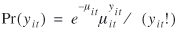 yit ∈ { 0,1,2,… } yit ∈ { 0,1,2,… }
In the generalized linear models context (GLM), the mean μit can be related to a vector of explanatory variables xit as μit = exp(x'it β) , or equivalently ln μit = x'it β (see McCullagh and Nelder 1989). Estimation of β can be performed by using the maximum likelihood (ML) estimator (see Maddala 1983; McCullagh and Nelder 1989).
A frequent problem in regression analysis, linear or nonlinear, is measurement errors in explanatory variables. Fuller (1987) gives an introduction to this subject for linear models and Carrol et al. (1995) treat the problem in the case of nonlinear models. The effect of measurement error in combination with multicollinearity in Poisson regression has been considered by Zidek et al. (1996). They demonstrate that the combination of measurement error and multicollinearity can cause misleading estimation results. The effect of important explanatory variables may be overlooked in an analysis, while the importance of other explanatory variables may be overstated.
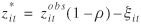
In the classical measurement-error model, the explanatory variables with measurement error are assumed to be measured as the true value plus an additive error. This model can be expressed as
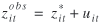
where
 denotes the observed value, denotes the observed value,
 denotes the true value, and denotes the true value, and
 is a random error term. is a random error term.
The other variables are assumed to be measured without error and are denoted by xit . In the Poisson regression case, the mean function can be written as
![uppercase e [ lowercase y vertical bar lowercase x subscript{lowercase i lowercase t}, lowercase z superscript{asterisk} subscript{lowercase i lowercase t} ] = exp [ lowercase x subscript{lowercase i lowercase t} lowercase beta plus lowercase z superscript{asterisk} subscript{lowercase i lowercase t} lowercase gamma ]](https://webarchive.library.unt.edu/eot2008/20090115161500im_/http://www.bts.gov/publications/journal_of_transportation_and_statistics/volume_09_number_01/images/Lundevaller-17.gif)
In the applied model,  is replaced by is replaced by  due to measurement errors and the mean of the applied model equals due to measurement errors and the mean of the applied model equals
![uppercase e [ lowercase y vertical bar lowercase x subscript{lowercase i lowercase t}, lowercase z superscript{obs} subscript{lowercase i lowercase t} ] = exp [ lowercase x subscript{lowercase i lowercase t} lowercase beta plus lowercase z superscript{obs} subscript{lowercase i lowercase t} lowercase gamma ]](https://webarchive.library.unt.edu/eot2008/20090115161500im_/http://www.bts.gov/publications/journal_of_transportation_and_statistics/volume_09_number_01/images/Lundevaller-20.gif)
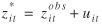
The measurement error uit can be expressed as
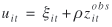
where 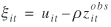 is not correlated with and ρ is a constant. This yields is not correlated with and ρ is a constant. This yields
Thus,
![uppercase e [ lowercase y vertical bar lowercase x subscript{lowercase i lowercase t}, lowercase z superscript{obs} subscript{lowercase i lowercase t}, lowercase z superscript{asterisk} subscript{lowercase i lowercase t} ] = exp [ lowercase x subscript{lowercase i lowercase t} lowercase beta plus lowercase z superscript{obs} subscript{lowercase i lowercase t} (1 minus lowercase rho) lowercase gamma minus lowercase xi subscript{lowercase i lowercase t} lowercase gamma ]](https://webarchive.library.unt.edu/eot2008/20090115161500im_/http://www.bts.gov/publications/journal_of_transportation_and_statistics/volume_09_number_01/images/Lundevaller-27.gif)
and
![uppercase e [ lowercase y vertical bar lowercase x subscript{lowercase i lowercase t}, lowercase z superscript{obs} subscript{lowercase i lowercase t} ] = uppercase e subscript{lowercase xi} [ exp [ lowercase x subscript{lowercase i lowercase t} lowercase beta plus lowercase z superscript{obs} subscript{lowercase i lowercase t} (1 minus lowercase rho) lowercase gamma minus lowercase xi subscript{lowercase i lowercase t} lowercase gamma ] ]](https://webarchive.library.unt.edu/eot2008/20090115161500im_/http://www.bts.gov/publications/journal_of_transportation_and_statistics/volume_09_number_01/images/Lundevaller-28.gif)
An indication of the combined effect of measurement error and multicollinearity can be obtained from this last expression. For instance, if xit and are independent and both and uit are normally distributed, then and ξit are independent and
![uppercase e [ lowercase y | lowercase x subscript{lowercase i lowercase t}, lowercase z superscript{obs} subscript{lowercase i lowercase t} ] = exp [ lowercase x subscript{lowercase i lowercase t} lowercase beta plus lowercase z superscript{obs} subscript{lowercase i lowercase t} lowercase gamma (1 minus lowercase rho) ] uppercase e subscript{lowercase xi} exp [ negative lowercase xi subscript{lowercase i lowercase t} lowercase gamma ]](https://webarchive.library.unt.edu/eot2008/20090115161500im_/http://www.bts.gov/publications/journal_of_transportation_and_statistics/volume_09_number_01/images/Lundevaller-35.gif)
Due to independence ,E ξ exp [ −ξit γ ] is not a function of xit or . Thus, estimation yields consistent estimates of slope coefficients in β and the coefficient γ (1 − ρ) .
Another situation is when xit and are independent, but the distributions of uit and are such that and ξit are dependent. Then E ξ exp [ −ξit γ ] is a function of , in general, and γ (1 − ρ) is inconsistently estimated while the estimator of the slopes in β is consistent. A third case is when and xit are correlated. This will cause both β and γ (1 − ρ) to be inconsistently estimated, in general, because the conditional expectation E ξ exp [ −ξit γ ] is a function of both and xit .
Another model is when the measurement errors can be written as
which is a simple form of what is often called the Berkson model (Carrol et al. 1995). This model is applicable, for example, in a controlled experiment where the administered doses are fixed but the actual uptake can vary randomly. Another example is if a distance variable is measured as the distance between two points on a map, while the relevant distance is the road distance.
If uit is independent of , then the mean of y conditional on xit and is
![uppercase e [ lowercase y vertical bar (lowercase x subscript{lowercase i lowercase t}, lowercase z superscript{obs} subscript{lowercase i lowercase t}) ] = exp [ lowercase x subscript{lowercase i lowercase t} lowercase beta plus lowercase z superscript{obs} subscript{lowercase i lowercase t} lowercase gamma ] uppercase e subscript{lowercase u} [ exp [ lowercase u subscript{lowercase i lowercase t} lowercase gamma ] ]](https://webarchive.library.unt.edu/eot2008/20090115161500im_/http://www.bts.gov/publications/journal_of_transportation_and_statistics/volume_09_number_01/images/Lundevaller-63.gif)
The Berkson measurement error model often makes it reasonable to assume that and uit are independent, which allows unbiased estimates of β and γ . However, if uit and are not independent, for example if is constant for all observations of an individual,  and uit are dependent on an individual, then γ will not be possible to estimate without bias. and uit are dependent on an individual, then γ will not be possible to estimate without bias.
TESTS OF RANDOM EFFECTS
In the case of repeated measurements, the assumption of independence may not be feasible, and observations within individuals tend to be correlated. One approach for modeling a correlation structure in repeated measurements data is to include a random individual specific component (random effect) in the linear predictor function. That is, let αi denote the random effect component, then the mean function is written as
μit = exp ( x'it β + αi )
(see Lindsey 1995). Note that this model is equivalent to a model with a multiplicative random effect (see Cameron and Trivedi 1998) because
μit = exp ( x'it β + αi ) = exp ( αi ) exp ( x'it β )
Inclusion of a random effects component into the model makes efficient estimation more complicated. The contribution to the likelihood from an individual is
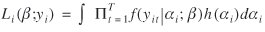
where h(αi) denotes the distribution of the random effects. In general, this integral is not analytically solvable. One exception is obtained if h(αi) is the gamma distribution, which is conjugate to the Poisson distribution. The integral can then be solved and standard methods of estimation are available. For other choices of h(αi) several analytical as well as simulation-based approximations have been suggested (see Cameron and Trivedi 1998). However, if the distribution of the random effects is treated as a nuisance component in the model, standard ML methods yield consistent but inefficient estimates of the coefficients in β, except for the intercept term (Liang and Zeger 1986).
Several tests of random effects have been proposed. Breusch and Pagan (1980) derive a score test (the BP test) for the linear regression model with normally distributed disturbances and random individual effects. Honda (1985) proposes the signed square root of the BP test statistic as a new statistic for the test of random effects. Honda's test is robust against nonnormality and is more powerful than the original BP test. Jacqmin-Gadda and Commenges (1995) propose a score test of random effects in GLMs.
For the Poisson regression model, the test statistic proposed by Jacqmin-Gadda and Commenges (1995) is

where

To obtain a statistic that is robust to overdispersion when φ is unknown, Jacqmin-Gadda and Commenges (1995) suggest the statistic

where
![lowercase phi caret is equal to summation with lowercase i of summation with lowercase t of lowercase u caret superscript{2} subscript{lowercase i lowercase t} [ summation with lowercase i of summation with lowercase t of lowercase mu caret subscript{lowercase i lowercase t} ] superscript{negative 1}](https://webarchive.library.unt.edu/eot2008/20090115161500im_/http://www.bts.gov/publications/journal_of_transportation_and_statistics/volume_09_number_01/images/Lundevaller-86.gif)
is a measure of overdispersion.
For the linear regression model, Häggström Lundevaller and Laitila (2002) propose the test statistic
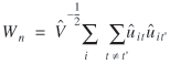
where
The test statistic is designed to be robust against potential heteroskedasticity. The simulation results reveal that the test works well for testing of random effects in the Poisson regression models considered here. All three statistics,  , Hφ , and Wn are compared with the standard normal distribution, and the null hypothesis is rejected for large positive values. , Hφ , and Wn are compared with the standard normal distribution, and the null hypothesis is rejected for large positive values.
These tests are derived to detect correlation that appears in random effects models. However, they are sensitive to correlation within individual observations regardless of the causes. Model misspecification that leads to correlation structures are likely to affect the tests. Here, the tests are applied to detect negative correlation.
SIMULATION STUDY
To evaluate the effect of measurement errors on bias of parameter estimates and tests of random effects, a simulation study was done. The idea of the simulations is to take a random sample from a large travel survey database and record the explanatory variables for the sampled observations. These sampled explanatory variables are then used to simulate new response variables employing estimates from the whole dataset as "true" parameters. Random individual effects and measurement errors can be introduced in the simulated model. The model is then re-estimated using simulated data and the effect of measurement error can be evaluated because we know the "true" values of parameters, random effects, and the measurement error.
Simulation Design
The data used in this simulation study are taken from the national travel survey (Statistics Sweden 1999); this survey is based on telephone interviews of samples of the Swedish population. The data were collected between April 1994 and December 1998 on a daily basis; 37,754 observations were recorded. The data collected consist of variables related to travel. The simulation study uses only observations with no partial nonresponse and with annual incomes of less than 900,000 SEK. The final dataset contains 30,775 observations.
Observations in the simulation study were obtained from the frequencies of purchase and recreational trips reported by the respondents. The individuals are indexed with i and trip purpose is indexed with t , where t = 1 denotes a recreational trip and t = 2 a purchase trip. Age (Age ), gender (Gen ), income (Inc ), and a price index for petrol (PP ) are used as explanatory variables. Both income and the index of petrol price are deflated by the consumer price index.
To assess the magnitude of multicollinearity, the multiple R 2 for each of these variables, using the other variables as explanatory variables is calculated. The results are 0.1838 (age), 0.0723 (gender), 0.2299 (income), and 0.0002 (petrol), which indicates a rather small multicollinearity problem. The model without measurement errors is as follows:
exp ( x'it β + αi ) = exp ( β0 DP + β1 DP Age + β2 DP Gen + β3 DP Inc + β4 DP PP + β5 DR + β6 DR Age + β7 DR Gen + β8 DR Inc + β9 DR PP + αi )
where D R is a dummy variable for recreational trips, D P is a dummy variable for purchase trips, and αi is the random effects component. The variables D P Age , D R Age , and so on denote the original variables multiplied by the dummy variable. The estimates of the model, assuming no random effects, obtained from the complete dataset are reported in table 1.
In the simulations, the parameters given in table 1 are used as the true parameters. A sample of 1,000 individuals was taken with replacement from the whole dataset, and the explanatory variables for these individuals are recorded. In the case of no measurement error, an observation of the response variable, yit , is created by calculating
where
 is the vector containing the estimates in table 1, is the vector containing the estimates in table 1,
xit is the vector with the explanatory variables drawn from the dataset, and
αi denotes random individual effects that are generated from the normal distribution with mean zero and standard deviation  . .
The levels of the standard deviation considered are = (0, 0.2, 0.4, 0.6). The value  is then used as the mean in a Poisson distribution from which an observation yit is generated by simulation. is then used as the mean in a Poisson distribution from which an observation yit is generated by simulation.
In the case of classical measurement errors, the procedure for generating data in the simulations is similar to the one described. However, the value of the explanatory variable is contaminated with an additive random error after the response variable yit has been generated.
Two of the explanatory variables are considered with measurement errors: the income and the petrol price index variables. The measurement errors for the petrol price index are generated as N(0, σP)
where
σP = (0.1μP, 0.2μP, 0.3μP)
where μP = 760.3 is the mean of the petrol price index over the observations. The measurements for income are generated as N(0, σP)
where σP = (0.1μP, 0.2μP, 0.3μP) and
μI =148534.6.
In the case of Berkson measurement errors, the value of the explanatory variable generated by sampling an observation from the dataset is stored and used in estimation. However, the simulated responses yit are generated by adding a random error term to the explanatory variable.
Applying the tests of random effects described earlier to the original dataset and the estimates given in table 1 yield the test statistic values = –8.84 and Wn = –8.72. Both these statistics are to be compared with the standard normal distribution. Because the tests are one-sided where evidence against the null hypothesis is found in large positive values, the null hypothesis of no random effects is not rejected. However, the test statistics are negative and indicate a negative correlation between the two response variables. A negative correlation can be motivated by, for example, time budget constraints (see Feather 1995).
For the study of the properties of tests of random effects under negatively correlated responses, one set of simulations are carried out where the random effect αi is added to the linear predictor for shopping trips,  , and the same value is subtracted from the linear predictor for recreation trips, , and the same value is subtracted from the linear predictor for recreation trips,  . Alternative models for generating negatively correlated responses could be used, but the chosen one is simple and is sufficient for the purposes of this study. . Alternative models for generating negatively correlated responses could be used, but the chosen one is simple and is sufficient for the purposes of this study.
Results
The results of the simulations are summarized in tables 2 and 3, which show the bias of the parameter estimates when measurement error exists. The sign of the true parameters is shown in a separate column. The results are for the case with no individual effects. The results observed with individual random effects, which are not shown here, are similar to those with no individual random effects. The measure of bias used is the mean of 100 ( −β)/|β| over the 2,000 replications. Parameters (β0−β4) are related to purchase trips and (β5−β9) to recreational trips and are taken from the estimation results using the whole table 1 dataset. −β)/|β| over the 2,000 replications. Parameters (β0−β4) are related to purchase trips and (β5−β9) to recreational trips and are taken from the estimation results using the whole table 1 dataset.
As expected, the simulation results shown in table 2 indicate only small bias under the Berkson measurement errors. In a few cases, especially for the estimates of the income and petrol price parameters, the values are not close to zero but there is no systematic pattern. This can also be seen in table 3 under the Berkson measurement errors where the bias estimates are generally close to zero with the exception of a few cases.
The results under classical measurement errors with measurement errors in petrol price in table 2 show a clear effect on the parameter estimates. The bias measures indicate that the estimates of the petrol price parameter are close to zero when measurement error exists. The intercept terms are also affected. These biased parameter estimates severely reduce the validity of the estimated model. The effect of classical measurement errors in income is less obvious (table 3). Here, a small tendency for the parameter estimates of the income variable to be closer to zero can be seen. The intercept terms are not much effected.
Table 4 shows the percentages of rejections observed at the 5% nominal significance level for the random effects test statistics in the case of explanatory variables with classical measurement errors. The distributions of measurement errors with the largest variances are compared with the case of no measurement errors. The results for the other levels of measurement error variances are similar and are not shown.
The results indicate that measurement error does not seriously affect the properties of the test statistics considered. The tests have estimated sizes close to the nominal sizes, and the estimated powers are high and increase with the variance of the random effects component.
For a study of the performance of the test statistics under negatively correlated responses, the tests were changed to employ double-sided alternative hypotheses. Results for the double-sided tests are shown in table 5, where rejection frequencies under negatively correlated response variables are considered. The table shows that the test statistics performed well according with rejection frequencies close to the nominal level when σα = 0 and an increasing power when σα = 0. The results show slightly higher rejection frequencies for the statistic Wn when σα is 0.2 or 0.4.
CONCLUSIONS
In this paper, the effect of measurement errors in explanatory variables in a travel frequency model is studied. Of major interest is the degree of bias introduced in the estimates of the Poisson regression. The derivations show that the effects of classical measurement errors are potentially more severe than those obtained from the Berkson type measurement errors. This result is also confirmed by the simulation results where only small relative biases are observed when Berkson errors are introduced.
The results are different for classical measurement errors. In this case, the intercept terms and the parameter estimates for the variable effected by measurement error are influenced by the measurement errors. This means that the parameter estimates for these variables are in serious doubt if classical measurement errors are suspected. The results for both Berkson and classical measurement errors confirm the findings in Zidek et al. (1996).
Problems due to the combination of multicollinearity and measurement errors are not observed in the results. The R 2 value for the regression of petrol price on the other explanatory variables is low, we do not expect any difficulty. The R 2 value for the income variable regressed on the other variables are a bit higher (0.2299), but still no effect can be observed.
Another problem that is addressed is the performance of tests of random effects in models of repeated measurement data under measurement errors in explanatory variables. The results suggest that the properties of the tests of random effects considered are not severely effected by measurement errors. The measurement errors are here assumed independent of the true explanatory variables.
The tests are also indicated to be potential candidates for tests of correlation of a more general form than the one obtained by the random effect specification. The properties of such tests under negative correlation among responses was studied. All statistics performed well in the simulations of negatively correlated response variables indicating that the tests can be used to test for negative correlation even though they have been suggested for positive correlation. Of special interest is the good performance of the test, Wn, proposed by Häggström Lundevaller and Laitila (2002). This test was initially derived for the linear regression case, but these results indicate that it can be used for Poisson regression also. However, further studies on the properties of the test in nonlinear models is needed.
ACKNOWLEDGMENTS
The author gratefully acknowledges the financial support from the Swedish Communications and Transportation Research Board and the Swedish Agency for Innovation Systems.
REFERENCES
Breusch, T.S. and A.R. Pagan. 1980. The Lagrange Multiplier Test and Its Applications to Model Specification in Econometrics. Review of Economic Studies 47:239–253.
Cameron, A.C. and P.K. Trivedi. 1998. Regression Analysis of Count Data.Cambridge, England: Cambridge University Press.
Carrol, R.J., D. Ruppert, and L.A. Stefanski. 1995. Measurement Error in Nonlinear Models.London, England: Chapman & Hall.
Feather, P. 1995. A Discrete-Count Model for Recreational Demand. Journal of Environmental Economics and Management 29:214–227.
Fuller, W. 1987. Measurement Error Models.New York, NY: Wiley.
Häggström Lundevaller, E. and T. Laitila. 2002. Test of Random Subject Effects in Heteroskedastic Linear Models. Biometrical Journal 44(7):825–834.
Hausman, J.A., G.K. Leonard, and D. McFadden. 1995. A Utility Consistent, Combined Discrete Choice and Count Data Model Assessing Recreational Use Losses Due to Natural Resource Damage. Journal of Public Economics 56:1–30.
Honda, Y. 1985. Testing the Error Components Model with Non-Normal Disturbances. Review of Economic Studies 52:681–690.
Jacqmin-Gadda, H. and D. Commenges. 1995. Tests of Homogeneity for Generalized Linear Models. J ournal of the American Statistical Association 90:1237–1246.
Le Cessie, S. and H.C. van Houwelingen. 1995. Testing the Fit of a Regression Model Via Score Tests in Random Effects Models. Biometrics 51:600–614.
Liang, K.-Y. and S.L. Zeger. 1986. Longitudinal Data Analysis Using Generalized Linear Models. Biometrika 73:13–22.
Lindsey, J.K. 1995. Modelling Frequency and Count Data.New York, NY: Oxford University Press.
Maddala, G. 1983. Limited Dependent and Qualitative Variables in Econometrics.Cambridge, England: Cambridge University Press.
McCullagh, P. and J.A. Nelder 1989. Generalized Linear Models. London, England: Chapman & Hall.
Statistics Sweden, Swedish Institute for Transport and Communications Analysis. 1999. National Travel Survey.
Zidek, J.V., H. Wong, N.D. Le, and R. Burnett. 1996. Causality, Measurement Error and Multicollinearity in Epidemiology. Environmetrics 7:441–451.
ADDRESS FOR CORRESPONDENCE
* E. Lundevaller, Department of Statistics, Umeå University, SE-901 87, Sweden. E-mail: erling.lundevaller@stat.umu.se
|