 |
||||
|
|
|
|||


|
|
Natural Recruitment of Salmonids in the Muskegon River, Michigan
This project is no longer current. Please see the Research Programs page for a list of current research projects.
Collaborators
Edward S. Rutherford, University of Michigan (UM
web site)
Mike Wiley, University of Michigan
Rationale: Sustainable harvest and management of the Great Lakes
 salmonid fisheries depends on accurate estimates of salmonid
adult abundance, recruitment, and harvest. Although recruitment of Lake
Michigan salmon and trout originally depended entirely on hatchery production,
significant natural reproduction of chinook salmon and steelhead now occurs
in Lake Michigan tributaries, and recently was estimated to contribute
at least 20-30% of the total adult population. Recent increases in natural
reproduction of anadromous salmonids may result from mandated changes
in hydropower operations that have improved salmonid nursery habitat below
hydropower dams. The increase in natural reproduction, combined with decreases
in natural mortality due to Bacterial Kidney Disease, and an increased
forage biomass of alewives, has permitted population biomass and harvest
rates of Lake Michigan chinook salmon to return to near-peak levels observed
during the early 1980's. The present record numbers of adult salmonids,
which during the 1980's depleted alewife forage and experienced high disease-related
mortality, have spurred managers to reduce hatchery production, and thereby
place greater importance on wild recruitment.
salmonid fisheries depends on accurate estimates of salmonid
adult abundance, recruitment, and harvest. Although recruitment of Lake
Michigan salmon and trout originally depended entirely on hatchery production,
significant natural reproduction of chinook salmon and steelhead now occurs
in Lake Michigan tributaries, and recently was estimated to contribute
at least 20-30% of the total adult population. Recent increases in natural
reproduction of anadromous salmonids may result from mandated changes
in hydropower operations that have improved salmonid nursery habitat below
hydropower dams. The increase in natural reproduction, combined with decreases
in natural mortality due to Bacterial Kidney Disease, and an increased
forage biomass of alewives, has permitted population biomass and harvest
rates of Lake Michigan chinook salmon to return to near-peak levels observed
during the early 1980's. The present record numbers of adult salmonids,
which during the 1980's depleted alewife forage and experienced high disease-related
mortality, have spurred managers to reduce hatchery production, and thereby
place greater importance on wild recruitment.
2005 Plans
Whereas past objectives focused on developing acoustics applications to quantify the number of naturally produced chinook smolts in Lake Michigan tributaries, this component focuses on understanding the sources of mortality for Chinook smolts while outmigrating. A significant source of smolt mortality is believed to be through walleye and northern pike predation on the outmigrating smolt. We hypothesize that the presence of alewife in Muskegon Lake and Muskegon River during the spring when smolts are outmigrating will buffer the predation pressure on the smolts, and thus the presence of alewife may indirectly benefit smolt survival. The objective of this sub-project is not to directly test the hypothesis, but rather to begin to understand the environmental cues that may lead to match/mis-match in timing between the smolt outmigration and the annual inshore spawning migrations of alewife into embayments an rivers, i.e., the spatial overlap between alewife, chinook smolt and potential predators. Specifically, we will determine the environmental cues that regulate the alewife inshore spawning migration in the spring and the cues that regulate the offshore movements of alewife later in the summer.
To achieve the above objective, we will quantify the abundance and spatial distribution of alewife in Lake Michigan and Muskegon Lake from April to October using hydroacoustics. Night acoustic transects will be performed twice a month starting at the northeast end of Muskegon Lake and will extend through the channel to the 110 m depth contour of Lake Michigan. Night sampling will be coordinated with the timing of the new and full moon. Such synchronous sampling with the lunar cycle will facilitate collaborations with another internal GLERL project by Scott Peacor (Trait mediated effects of invasive predatory cladocerans). Acoustic data will be shared with Peacor. CTD profiles will be performed along the acoustics transect to map thermal structure. These data will be used to develop a model to predict the timing of the alewife spring inshore spawning migration.
2004 Progress
Pre-smolt and smolt abundance from electrofishing and smolt trap
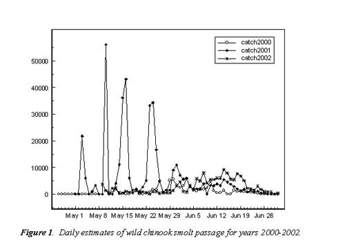
2000. Pre-smolt surveys and smolt trapping indicated natural recruitment of chinook salmon in 2000 was low compared to historic estimates. The pre-smolt abundance estimates indicated 100,000 wild pre-smolts were available to leave the Muskegon River by early May. This estimate compares to 350,000 estimated by Carl (1982) in 1979, and an estimated 284,000 pre-smolts estimated by O’Neal (1988) in 1988. Smolts estimated from catches in the smolt trap from late 27 April – 30 June indicated a total of 70,000 smolts left the river. The peak of the chinook smolt migration occurred during the late June 3rd (Figure 1). Majority of the smolts began out-migrating when water temperatures ranged between 13° and 20°C (Figure 2A). Efficiency of the smolt trap was estimated at 2.8%.
2001. Pre-smolt surveys and smolt trapping indicated
natural recruitment of chinook salmon in 2001 was high and comparable
to historic estimates. The pre-smolt early May abundance estimates (electrofishing
survey) indicated 857,840 wild pre-smolts were available to leave the
Muskegon River. This estimate compares to 350,000 estimated by Carl (1982)
in 1979, and an estimated 284,000 pre-smolts estimated by O’Neal
in 1988. Smolts estimated from catches in the auger trap from 2 May -
26 June indicated 384,000 smolts left the river; approximately 45% May
10th compared to early June in 2000 (Figure 1). Majority of smolts began
out-migrating when water temperatures ranged between 13 and 18°C (Figure
2B). Efficiency of the auger trap was estimated at 1.85 %, which was lower
than last year’s estimate and previous efficiency estimates of 3-5%
made using this trap in the Au Sable River in 1999 and Manistee River
in of the estimated number of pre-smolts. The peak of the chinook smolt
migration occurred during 1998. The lower efficiency in 2001 was likely
a result of extremely high river discharge.
2002. Chinook salmon passage over the course of the 2002
field study was estimated to be 137,150 identified wild chinook smolts.
Our 2002 estimate of wild fish is approximately twice that estimated in
2000 (69,000 smolts) and less than half of that estimated for 2001 (384,000
smolts). The peak of the migration occurred on June 14 (9,205 out-migrants).
This is the latest peak observed in this study, with the 2000 and 2001
peaks occurring in June 3 and May 10 respectively (Figure 1). Majority
of smolts out-migrated when water temperature ranged between 13 and 20°C,
similar to the 2 previous (Figure 2C). We estimated trap efficiency at
1.26% in 2002.

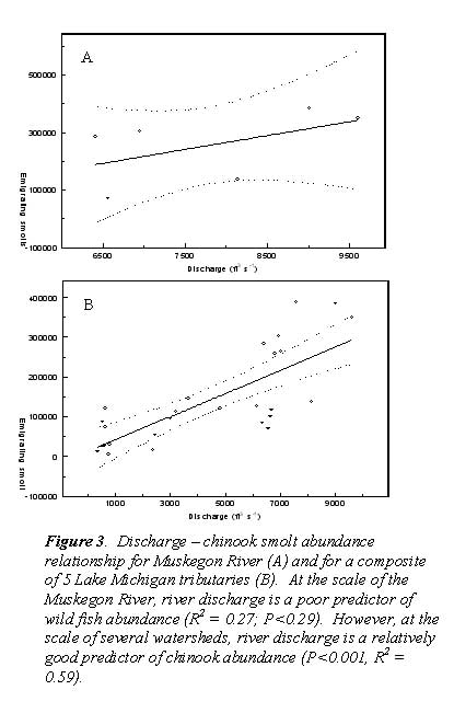
Differences between historic and present survey estimates of chinook smolt abundance may be explained by annual variability in river discharge. Chinook recruitment has been positively correlated with river discharge in the Pere Marquette River (Zafft 1992) and in west coast populations. Muskegon River discharge from mid-March to June was extremely high (8,994 ft3 s-1) compared to discharge of 9,590 ft3 s-1 estimated during 1979, a year of high recruitment. Discharge was near a period-of-record low (6,557 ft3 s-1) in 2000 when we observed a low recruitment. Regression analysis of observed chinook recruitments in the Muskegon River indicated a positive but non-significant relationship (P<0.29, R2 = 0.27) between recruitment and discharge (Figure 3A). However, when Muskegon River data were averaged and compared with recruitment data for other Lake Michigan tributaries, there is a significant positive relationship (P<0.001, R2 = 0.59) between chinook recruitment and discharge (Figure 3B).
Hydroacoustic estimates of fish passage
Table 1 shows the daily passage rate by range, and the auger trap estimates for the same dates. Daily estimates differed between the auger smolt trap and the hydroacoustics. In 2001, the hydroacoustic estimates where generally higher by a factor 3-12 times. However in 2002, estimates where in the same general range, but at times differed on specific dates. Despite differences in absolute passage rages, the relative changes in daily passage rates where similar (Figure 4). In 2001, fish passage estimates peaked for both gears within a couple days of one another (June 13 and 14) and declined there after. In 2002, peak densities for both gears occurred on June 7, but the acoustics measured a potentially earlier peak in out-migration not observed in from the smolt trap.
Table 1. Hydroacoustic and trap-based chinook smolt passage rates (number of smolt per day) for specific dates in 2001 and 2002. Distance measures for hydroacoustic estimates represent estimates from 0-5m from the transducer, 0-10m from transducer, etc.
| Date | Trap Estimates |
Hydroacoustics estimates by range (m)
|
||||
0-5 |
0-10 |
0-15 |
0-20 |
Entire River |
||
| 2001 | ||||||
6/8 |
4,000 |
2,087 |
2,792 |
5,311 |
6,888 |
12,199 |
6/10 |
3,351 |
1,166 |
2,399 |
4,683 |
5,296 |
9,979 |
6/11 |
3,135 |
1,980 |
5,847 |
9,531 |
10,322 |
19,854 |
6/12 |
3,838 |
2,947 |
7,272 |
15,968 |
16,917 |
32,886 |
6/13 |
3,189 |
2,916 |
6,568 |
12,440 |
12,920 |
25,360 |
6/14 |
5,459 |
1,872 |
3,657 |
7,395 |
8,021 |
15,416 |
6/19 |
1,243 |
1,128 |
3,482 |
4,213 |
4,319 |
8,532 |
6/20 |
1,838 |
1,473 |
4,566 |
5,476 |
5,787 |
11,263 |
6/21 |
919 |
660 |
2,196 |
2,949 |
3,122 |
6,071 |
6/22 |
1,405 |
1,328 |
2,664 |
2,689 |
2,736 |
5,424 |
6/23 |
865 |
3,645 |
5,401 |
5,455 |
5,551 |
11,006 |
| 2002 | ||||||
5/26 |
317 |
246 |
805 |
1,099 |
1,346 |
2,444 |
5/29 |
556 |
752 |
1,614 |
2,168 |
2,544 |
4,712 |
5/30 |
1,349 |
706 |
1,330 |
1,738 |
1,923 |
3,662 |
5/31 |
3,095 |
760 |
1,283 |
1,424 |
1,540 |
2,964 |
6/5 |
1,825 |
576 |
1,601 |
1,913 |
2,105 |
4,018 |
6/6 |
5,793 |
591 |
1,373 |
1,756 |
2,063 |
3,819 |
6/7 |
4,920 |
990 |
1,946 |
2,522 |
3,194 |
5,715 |
Comparison between gear types
Estimates of smolt passage from smolt trap and hydroacoustics where significantly positively correlated within years and when years were combined (Figure 5). In general, the hydroacoustics estimated a greater number of smolts out-migrating then the auger smolt trap.


Figure 5. Regression (with 95% confidence intervals) between Log10 transformed smolt passage estimates from smolt trap and hydroacoustics. 2001- P=0.024, R2= 0.44; 2002-P=0.08, R2=0.30 ; Years combined- P=0.067, R2=0.19.
Previous Accomplishments
Objective 1: To evaluate the feasibility of using fixed-location riverine
hydroacoustics technology to measure smolt abundance.
Digital signal processing of raw acoustics data is underway. As a first
step to automating the signal processing, we have evaluated the accuracy
with which the automated processing protocol generates results relative
to visual inspection of the raw data from color echograms. It is critical
that the automated process be developed as 10's of Gigabytes of data can
be expected to be collected in a given year (e.g., 25 Gigabytes in 2001
and 31 Gigabytes in 2002).
Methods: We are using the software Echoview 2.25.60 for the digital signal processing. Raw data echograms consisting of 1 hour of acoustic data were displayed and inspected for traces (Figure 6). A trace is defined as series of echoes from a sequence of pings that progress in a predictable manner. When a potential trace is identified, the user outlines the trace with a polygon. This polygon serves as a marker region for spatio-temporal comparisons between expected and observed fish tracks.
Following the complete inspection and identification of all suspected traces within the raw echogram, the Single Target Detection Algorithm (STDA) in the software is applied to the data. The STDA is a process that identifies echoes that meet specific criteria indicating quality data. These include: acoustical target strength (TS), echo pulse width, angles off the acoustic axis, and precision of the angle measurements. An analysis of the algorithm's criteria was conducted to determine the value to be used for each individual criterion. The STDA creates a single target variable that contains information on all echoes that pass the algorithm's criteria.
Echoview's Fish Tracking Algorithm (FTA) is then applied to the single target variable. The FTA analyzes the single target variable by a process called candidature. When the algorithm encounters a single target, a fish track is opened. Echoview then searches for echoes that are likely to be associated with the opening target. An ellipsoid is created to predict the 3-dimensional location of the target on the next ping. If a target falls within that ellipsoid, it is added to the track, and the algorithm repeats this process for the next ping. If no target is identified, the algorithm moves to the next ping, increasing the dimensions of the ellipsoid by a user-specified percentage. This process will continue until the maximum ping gap parameter is exceeded. When the maximum ping gap has been reached, the track is closed. Tracks including multiple targets are defined as regions. Export of information about the track, such as TS and spatial data, is then done for further analysis.

Figure 6. 2.5 minute echogram showing echo traces, tracks, and polygons. Top of the image represents the shoreline out side ways about 20 meters. All marks from the shoreline to 20 meters distance from the shoreline are echo traces. Echo tracks identified by the software are labeled. Orange polygons are user-defined fish tracks (expected fish tracks) based simply on looking at the echo traces. Dark single traces are representative of the background noise in the river.
Objective 2: To quantify smolt behavior during migration. Preliminary data from the acoustics suggest that migratory behavior of Chinook smolts tends to peak in late afternoon, drop and remain relatively constant at night, and then declines to a minimum during the daylight hours (Figure 7).

Figure 7. Proportion of smolts counted per hour - averaged over 6 days
Objective 3: To estimate abundance of out-migrating smolts. We compared the preliminary acoustics
estimates to the chinook abundance estimates obtained from the smolt trap
(Figure 8). Acoustic estimates appeared to provide realistic estimate
of chinook smolts, despite the issues that still need to be resolved in
the automated fish counting procedure. Acoustics estimates tended to be
higher than estimates derived from the smolt traps when trap estimates
where low; but this relationship was reversed for when trap estimates
where high. During the same two-week period, size estimates of outmigrating
smolts from both the acoustics and from fish collected in the smolt trap
remained relatively the same (Figure 9).
We compared the preliminary acoustics
estimates to the chinook abundance estimates obtained from the smolt trap
(Figure 8). Acoustic estimates appeared to provide realistic estimate
of chinook smolts, despite the issues that still need to be resolved in
the automated fish counting procedure. Acoustics estimates tended to be
higher than estimates derived from the smolt traps when trap estimates
where low; but this relationship was reversed for when trap estimates
where high. During the same two-week period, size estimates of outmigrating
smolts from both the acoustics and from fish collected in the smolt trap
remained relatively the same (Figure 9).

Figure 8. Number of smolts outmigrating. Derived from the smolt trap estimates vs. acoustic counts for 7 days ranging from end of May through the beginning of June. Dotted line is the 1:1 line, where acoustic estimates are the same as the trap estimates.
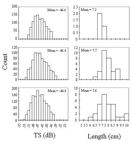
Figure 9. Estimates of smolt size from acoustics (left) and smolt trap (right) on three different dates- May 26, May 31, and June 7, 2002.
Sampling for smolt
Products
Great Lakes Fishery Trust Completion report: Project No. 1999.9
Salmonid spawning stock
abundance, recruitment and exploitation in the Muskegon River.