Contact Us Search: All EPA This Area

• You are here: EPA Home
• Research & Development
• National Center for Environmental Research
• Research Project Search
• Demographic Change in the New West: Exurban Development Around Nature Reserves
• Final Report

Research Project Search

 Enter Search Term:
   
 NCER Advanced Search

Final Report: Demographic Change in the New West: Exurban Development Around Nature Reserves

EPA Grant Number: R828786
Title: Demographic Change in the New West: Exurban Development Around Nature Reserves
Investigators: Hansen, Andrew , Maxwell, Bruce , Rasker, Ray
Institution: Montana State University
EPA Project Officer: Jones, Brandon
Project Period: May 1, 2001 through April 30, 2003 (Extended to April 30, 2004)
Project Amount: $400,000
RFA: Futures Research in Socio-Economics (2000)
Research Category: Economics and Decision Sciences

Description:

Objective:

The overall objective of this research project was to develop a means to model and evaluate past and future rural development in the Greater Yellowstone Ecosystem (GYE). The specific objectives of this research project were to: (1) determine socioeconomic and ecological predictors of rural development among and within communities of the GYE; (2) construct the rural development simulator (RDS) and parameterize the model with the results from objective 1; (3) use the RDS to simulate three alternative future scenarios of rural development across the GYE; and (4) demonstrate a method of assessing ecosystem vulnerability to rural development.

Summary/Accomplishments (Outputs/Outcomes):

Rates and Drivers of Rural Residential Development

The factors driving rural development across the United States are thought to have evolved with human technology. One proposed paradigm of the drivers of human settlement describes three stages characterized by: (1) natural resource constraints; (2) transportation expansion; and (3) pursuit of natural amenities (Huston, in review; Riebsame, et al., 1996; Wyckoff and Dilsaver, 1995; James, 1995). We evaluated the validity of this model for explaining past rural residential development (RRD) patterns in the GYE. Our hope is that an improved understanding of how and why development patterns occur will allow rural communities in the GYE and similar regions to manage residential development in a manner than minimizes ecological and socioeconomic costs without limiting overall growth.

Time Frame and Spatial Extent

We compiled a spatially explicit database of rural homes, describing the locations of all known rural homes and the years in which they were built within the 20 counties of the GYE (Figure 1). Rural homes are defined as all homes that are outside of incorporated city and town site boundaries, including subdivisions and excluding mobile homes. The data were collected from County Tax Assessors offices and State Departments of Revenue and are summarized per section, within township range blocks, according to the U.S. Public Land Survey System. The resolution of the database is therefore the area of a section, approximately 2.59 square kilometers. For any given section within the study area, the database describes the number of rural homes present during each year, from 1900 through 1999.

Figure 1. The Study Area Encompasses Those Twenty Counties of Montana, Wyoming, and Idaho That Surround Yellowstone National Park. The public and tribal lands shown comprise 68 percent of the region.

Modeling Approach and Results

Accuracy Assessment of Response Variable. We conducted an accuracy assessment of the rural homes dataset using aerial photography. Within a sample of 76 sections, we compared the number of rural homes reported by the dataset to the number from aerial photographs. The sections were sampled in six GYE counties in locations where post-1994 aerial photographs were available. The mean difference in counts of rural homes was 0.17 homes per section (std. dev. = 1.65). Using a paired t-test, we failed to reject the hypothesis that the mean differences in counts between the dataset and the aerial photographs was zero (P = 0.37). Thus, we maintain a high degree of confidence in the tax assessor rural homes data.

Rural Residential Development 1900-1999. We evaluated the role of natural resource constraints in driving patterns of RRD (1900-1999); in particular, the assertion that growth during the early 1900s was a function of the distribution of natural resources and that this relationship has weakened as technology allowed people to live greater distances from these resources. We used spatially explicit datasets describing agricultural suitability and distance to surface water to denote natural resource constraints. The agricultural dataset was calculated as the mean nonirrigated capability class per the U.S. Department of Agriculture state soil geographic (STATSGO) map unit and rates suitability as a function of soil, topographic, and climatic characteristics. The hydrology dataset describes Euclidian distance to surface water as delineated in the National Hydrography Dataset (NHD) 1999 database. The NHD is based on the USGS 1:100,000-scale Digital Line Graph data, integrated with information from the U.S. Environmental Protection Agency Reach File Version 3.0.

We divided the 1900s into four even time periods (1900-1925, 1925-1950, 1950-1975, and 1975-1999) and employed a use versus availability analysis per time period to examine the distribution of homes built within each period with respect to agricultural suitability and access to water. As expected, during the early 1900s, home sites were disproportionately located in highly productive soils and lands proximate to water. Although we expected this relationship to weaken over time, it remained consistent throughout the four time periods considered. For each period, we rejected the hypotheses that rural homes were distributed randomly with respect to soil productivity and proximity to surface water (P < 0.001).

Rural Residential Development 1970-1999. We evaluated the role of natural resources, infrastructure and services, natural amenities, and past development in driving recent growth patterns (1970-1999). The time period considered for this analysis was selected because of the acceleration in RRD since 1970, and because of the lack of available pre-1970 spatial datasets to represent these concepts, in particular infrastructure and services. Specific hypotheses for describing recent patterns of development in the GYE are as follows:

Hypothesis 1 (H1): Recent growth in RRD is strongly related to the distribution of natural resources.
Hypothesis 2 (H2): RRD in recent decades was driven by transportation infrastructure and associated services.
Hypothesis 3 (H3): The locations of rural homes reflect proximity to natural amenities.
Hypothesis 4 (H4): Past development promotes further growth by affecting accessibility and land markets.
Hypothesis 5 (H5): The grouping of factors that most accurately describes trends in RRD (1970-1999) accounts for the combined effects of H1, H2, H3, and H4.

The response variable for evaluating these hypotheses was the change in rural homes per square mile section over the time period 1970-1999. Several explanatory variables were compiled for use in evaluating these hypotheses (Table 1). One-quarter of private lands in the study area, a randomly selected 6217 sections, were excluded from model building for use in assessing model accuracy. For the remaining sections, we used generalized linear models (GLM) with the assumption of a negative binomial distribution (SAS Institute Inc., 2001) and a log link.

Table 1. Potential Covariates of Growth in RRD From 1970 to 1999 Were Compiled from the Listed Sources. Federal agencies from which data were acquired are abbreviated (DA = Department of Agriculture, CB = Census Bureau, GS = Geological Survey, DOT = Department of Transportation, EPA = Environmental Protection Agency). Exploratory selection results are provided for the univariate models of growth in RRD from 1970-1999. Explanatory variables within each category (natural resources, transportation, services, etc.) were ranked according to Delta AIC values.

ª Tabular source data, such as U.S. Census figures, were joined to spatial datasets with the listed scale.
^b Sources included the Montana Natural Heritage Program, the University of Wyoming Spatial Data and Visualization Center, and the Idaho Cooperative Fish and Wildlife Research Unit.
^c AIC weights equal 1 for these factors and 0 for the remaining factors within the same class.
^d Factors not redundant with the highest ranked factor within the same class, which were selected for use in model comparisons.

We used exploratory analyses to identify those datasets within each of six classes that explained the most variation in growth in RRD (Table 1). Within each class, all variables were fit to the response data using univariate GLM. The variables selected in exploratory analyses were used to build four statistical models (representing H1-4) of growth in RRD. To test H5, the four statistical models representing H1, H2, H3, and H4 were grouped in all possible combinations and ranked according to Akaike’s Information Criteria (AIC) (Burnham and Anderson, 2000). Among all possible combinations of models, there was clear support for one model according to the Akaike weights. This model (representing H5) incorporated agricultural suitability, past development, transportation infrastructure, and accessibility to services, as well as the effects of towns and natural amenities. To test for spatial autocorrelation, Pearson residuals from the best model were mapped and plotted in variograms. No spatial pattern was evident in the map of Pearson residuals, and the variogram showed only weak spatial autocorrelation. It is therefore likely that the combined model (H5) captured the relevant covariates to explain the spatial patterns in RRD.

The best model was run for the excluded sections, and errors of over and underestimation were calculated. The mean difference between predicted and observed growth in number of rural homes per section was -1.18 homes (std. dev. = 9.59). Of the 6217 sections evaluated, the increase in the number of rural homes was correctly predicted for 80 percent (4953 sections). Of those sections in which growth was underestimated (104 sections), the mean difference was seven homes. Of the sections in which growth was overestimated (1160 sections), the mean difference was four homes. Using a paired t-test, we failed to reject the hypothesis that the mean of the differences between observed and predicted change in rural homes was zero (P = 0.11).

Simulation of Future Rural Residential Development

Goal. There is a growing need to support local decisions about the impacts of development on local economies and the environment. Analytical tools for simulating future growth are needed so that local governments can visualize growth scenarios and make decisions with a more complete understanding of the consequences. In the GYE there are vast amounts of undeveloped land, unrestrictive land use policies, and generally underfunded and understaffed county planning departments. Thus, there exists high potential for undirected and unmanaged growth on the private lands surrounding one of the nation’s most well-known nature reserves. Our objective for this portion of the study was to simulate alternative future scenarios of rural development in the GYE.

Time Frame and Spatial Extent. Four alternative scenarios were generated for all 24,999 square mile sections containing private lands within the GYE for the years 2010 and 2020. These scenarios were based on the rates and spatial patterns of RRD that occurred during the 1990s.

Modeling Approach and Results. Differences in the relationships between explanatory variables (Table 1) and RRD patterns among portions of the GYE were assessed by visually examining univariate plots. This was necessary to determine if regions of the GYE should be modeled separately. The plots showed that correlates of growth did not differ between regions; therefore, our next step was to identify the variables that explained the most variation in growth in RRD within the GYE as a whole.

Again, one-quarter of private lands in the study area, a randomly selected 6217 sections, were excluded from the analysis as a hold-back dataset for use in assessing model accuracy. For the remaining sections, the potential explanatory variables were fit to the response variable (change in number of rural homes per section during the 1990s) using univariate GLMs. Within each of the six categories (Table 1), those variables that explained the most variation in growth in RRD during the 1990s were identified. All possible combinations of the selected variables were ranked according to differences in AIC scores, and the best model was identified (Table 2).

Table 2. Coefficient Estimates, Confidence Limits, and Significance Levels for the Best Model (Delta AIC = 0) Parameters

Model Parameters	β	95% Confidence Limits	P-value
Intercept	9.02	7.39, 10.73	<.0001
Road Density	3.01	2.53, 3.49	<.0001
Airport Travel Time	-0.65	-0.98, -0.34	<.0001
Development Indicator	1.75	1.65, 1.86	<.0001
Homes in 1 Section Radius	3.80	3.12, 4.52	<.0001
Homes in 20 Section Radius	0.16	0.03, 0.30	0.0203
Homes in 20 Section Radius - Quadratic Term	-0.89	-1.12, -0.66	<.0001
Construction During Previous Decade	9.76	8.14, 11.47	<.0001
Streams/ Rivers Proximity	-1.12	-1.33, -0.92	<.0001
Forest Areas Travel Time	-3.31	-3.58, -3.03	<.0001
Dispersion		3.67	3.46, 3.89

We found no evidence of spatial autocorrelation in the residual variation in the best model. This model was run for the hold-back dataset, and the mean difference between predicted and observed growth in number of rural homes per section was 0.14 homes (std. dev. = 3.92). The increase in number of rural homes was correctly predicted for 83 percent of sections, and correctly predicted to plus or minus one home in 94 percent of sections. In sections where growth occurred during the 1990s, the mean percent deviation was 7.31 percent.

Using the best GLM of growth during the 1990s, the RDS was run for two iterations of one decade each to forecast development patterns for 2010 and 2020 (Figure 2). Specifically, the RDS, which consists of interacting Java and ARC/INFO programs, was used to implement zoning and other growth management (GM) regulations that affected allowable housing densities, and to calculate the past development variables that were used as model inputs.

Figure 2. The Best Model Was Run Iteratively to Forecast RRD for the Years 2010 and 2020

The RDS was designed to facilitate the manipulation of growth inducing and limiting factors to generate maps of alternative future scenarios. Four alternative scenarios were generated for the purpose of visualizing the potential for growth in the GYE and assessing existing and hypothetical GM policies (Table 3).

Table 3. The Future Growth Scenarios Generated By the RDS Use Different Assumptions of Growth Rates, Limiting, and Driving Factors

Simulation Assumptions
Scenario	Years Simulated	Rate of Rural Home Construction	Limiting Factors	Driving Factors
Status Quo	2010, 2020	Point estimates of coefficients from best model	Existing zoning districts and conservation easements	Covariates from best regression model
Low Growth	2010, 2020	Lower coefficient estimates from 95% confidence limit	Existing zoning districts and conservation easements	Covariates from best regression model
Boom	2010, 2020	Upper coefficient estimates from 95% confidence limit	Existing zoning districts and conservation easements	Covariates from best regression model altered to reflect hypothetical gains in transportation and housing
Growth Management	2010, 2020	Point estimates of coefficients from best model	Existing and hypothetical zoning districts and conservation easements	Covariates from best regression model

The mathematical models for all four scenarios were in the form of linear equations; however, forecasted growth was nonlinear (Figure 3) because of the influence of the past development variables.

Figure 3. The RDS Was Used to Forecast RRD for the Years 2010 and 2020

In both the status quo (SQ) and GM scenarios, the number of rural homes within the GYE was forecasted to increase by 82.38 percent from 1999 to 2020. Although the increase in rural housing was forecasted to be the same between these scenarios, the distribution differed as a result of the hypothetical zoning districts and conservation easements implemented in the GM scenario. In the low growth (LG) scenario, an increase of 27.51 percent was forecasted to occur, and in the boom (BM) scenario an increase of 233.63 percent was forecasted to occur.

In the SQ, LG, and BM scenarios, the forecasted homes were disproportionately distributed near protected areas and towns mainly in the northern and western portions of the study area. Differences between the SQ and GM scenarios were concentrated in areas ranked as high priorities for biological conservation (Figure 4). In the GM scenario, conversion from low to exurban housing densities of greater than one home per 16.2 hectares (Brown, et. al, in review) was forecasted to occur in 3298 fewer sections than in the SQ scenario. Although the number of forecasted homes in the GM and SQ scenarios was equal, growth in the GM scenario was more concentrated in already developed sections resulting in less conversion of natural and agricultural lands (Table 4).

Figure 4. Red Polygons Represent Core Areas of More Forecasted Growth Than in the 2020 SQ Scenario, and Blue Polygons Represent Core Areas of Less Forecasted Growth Than in the 2020 SQ Scenario

Table 4. The Percent Increase in Types of Land Use Changes Differed Between the Four Scenarios. Hypothetical GM policies implemented in the GM scenario resulted in the conservation of undeveloped land and land currently occupied at low housing densities.

Forecasted Land Use Change
in GYE Private Lands of High Conservation Priority
Scenario	Low Density to Exurban	Undeveloped to Developed
Low Growth	4.70%	4.58%
Status Quo	14.56%	7.66%
Boom	36.37%	24.29%
Growth Management	1.37%	3.07%

Assessment of Habitat and Biodiversity Consequences

Goal. The development of rural lands is the result of many decisions made by individual landowners and local governments (Theobald, 2000), resulting in patterns of growth that may negatively impact greater ecosystems. The objective for this part of the study was to conduct a regional assessment of ecological consequences of alternative future development scenarios. This approach could be incorporated in an adaptive management framework to help managers visualize the impacts of alternative policies and select policies that balance biodiversity and growth objectives.

Time Frame and Spatial Extent. Data representing land cover types, species distributions, and biodiversity indices were collected for the GYE and overlaid with maps of the distribution of rural housing for the years 1900, 1972, and 1999 and alternative scenarios of forecasted rural housing in 2020.

Modeling Approach and Results. We collected three categories of habitat and biodiversity response variables for the GYE: (1) land cover data, (2) species/habitat data, and (3) biodiversity indices (Table 5).

Table 5. Response Variables Considered in the Assessment of Habitat and Biodiversity Consequences of Past and Present Rural Development, and Future Rural Development Scenarios

Response	Description	Source	Scale
Land Cover Types
Douglas Fir	As classified by USGS.	GS 1992 National Land Cover	1:24,000
Grassland	As classified by USGS.	GS 1992 National Land Cover	1:24,000
Aspen	On public lands, as classified by USFS; Else, deciduous excluding riparian.	GS 1992 National Land Cover; 1990-2001 USFS Stand Maps	1:24,000
Riparian	Major rivers buffered by 256m and adjacent deciduous habitat.	GS 1992 National Land Cover; GS/EPA 1999 Hydrography; USFS 1900-2001 Stand Maps	1:100,000
Species Distributions
Grizzly Bear	Outer edge of composite polygon of fixed kernel ranges from all grizzly locations (1990-2000).	Shwartz et al. 2002	1:24,000
Elk Winter Range	Habitat suitability; Expert opinion.	RM Elk Foundation 1999	1:250,000
Pronghorn Antelope	Habitat suitability; Expert opinion.	MT FWP 2002; WY G&F	1:250,000
Moose	Habitat suitability; Expert opinion.	MT FWP 1996; WY G&F	1:250,000
Biodiversity Indices
Bird Hotspots	Areas of > 70% of maximum bird diversity and abundance.	Hansen et al. 2003	1:250,000
Migration Corridors	Landscape corridors based on habitat suitability for grizzly, elk, and cougar.	Walker and Craighead 1997	1:250,000
Irreplaceable Areas	Multi-criteria assessment based on habitat and population data for terrestrial and aquatic GYE species.	Noss et al. 2002	1:250,000

For each response, we calculated the proportion of area impacted by various rural housing densities in 1900, 1972, and 1999 and the alternative scenarios in 2020. The years 1900 and 1972 represent conditions prior to the BM in RRD. Two classes of rural housing densities were considered: low densities at less than one home per 16.2 hectares, and exurban densities of greater than one home per 16.2 hectares. This threshold is meaningful because at exurban densities, areas are generally considered to be more populated than working agricultural lands (Brown, et. al, in review). If responses occur within the same section as low density housing or within one section of exurban housing, they are considered impacted. We found that for all responses, the area affected by low density rural housing is decreasing as low density housing is converted to exurban housing (example, Figure 5). Of the response variables considered, riparian areas, bird hotspots, and migration corridors (Figure 6) are the most at risk of development. For these response variables, more than 20 percent of their total area is forecasted to be impacted by RRD by 2020 (Table 6).

Figure 5. The Proportion of Riparian Areas Impacted By Low Density RRD Is Decreasing, and the Proportion Impacted By Exurban Densities of Rural Housing Is Increasing

Table 6. For Each Response, We Calculated the Percent of Total Area Impacted By Exurban Development. The percent of private land area impacted by exurban development is included in parentheses.

Percent of Area Impacted by Exurban Development
Response	1972	1999	GM 2020	SQ 2020
Land Cover Type
Douglas Fir	1.69% (3.16)	5.80% (13.89)	7.31% (17.81)	8.34% (18.91)
Grassland	1.26% (1.91)	4.89% (7.82)	6.47% (10.64)	6.89% (11.01)
Aspen	1.53% (2.86)	9.67% (15.06)	12.69% (19.07)	14.00% (20.36)
Riparian	5.12% (7.28)	16.37% (24.73)	19.97% (30.77)	22.10% (33.40)
Species Distribution
Grizzly Bear	1.50% (3.22)	4.61% (18.57)	5.27% (21.97)	6.10% (24.7)
Elk Winter Range	1.37% (1.30)	5.46% (7.53)	6.91% (10.00)	7.66% (10.50)
Pronghorn Antelope	0.55% (0.74)	2.49% (4.05)	3.42% (5.91)	3.51% (6.09)
Moose	1.35% (3.05)	4.83% (13.85)	6.13% (18.17)	6.76% (19.07)
Biodiversity Indices
Bird Hotspots	4.38% (5.08)	16.54% (21.54)	20.32% (26.76)	22.38% (28.42)
Migration Corridors	3.85% (3.90)	17.19% (16.69)	21.96% (21.45)	22.4% (21.85)
Irreplaceable Areas	2.64% (4.49)	9.09% (20.79)	10.54% (24.7)	11.71% (26.34)

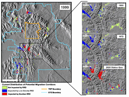
Figure 6. Potential Migrations Corridors for Grizzlies, Elk, and Cougar Are Heavily Impacted By Both Low Density and Exurban Housing in the Rural GYE

We analyzed use versus availability for each response to assess whether RRD was occurring disproportionately in ecologically sensitive areas (example, Figure 7). For all responses, with the exception of elk and pronghorn antelope ranges, we found that rural homes built between 1900 and 1999 disproportionately overlapped with the responses. Pronghorn habitat consists of dry sagebrush habitat in the northern and southeastern portions of the study area, which tend to be less scenic, and conservation of elk habitat has been a success in Montana in particular. For all responses, the GM scenario, in which growth was more concentrated, resulted in better conservation of the response variables (Table 6).

Figure 7. The Location of Rural Homes Is Shown Relative to the Current Distribution of Aspen. Expected values are proportional to the area of aspen.

Implications and Current Users

Implications of Historical Analyses of Rural Residential Development. Our analyses support that three stages of human settlement (natural resource constraints, transportation expansion, and pursuit of natural amenities) have shaped patterns of RRD within the GYE. Additionally, our research suggests that each phase of development has left a legacy upon the landscape, and that factors that drove early settlement patterns remain strongly correlated with patterns of land use today.

The patterns of RRD we have described potentially threaten biodiversity within the Yellowstone and Grand Teton National Parks. Our results suggest that RRD has occurred disproportionately on lands bordering the parks. This configuration of RRD may result in a barrier between wildlife and the lowland habitats on which they depend. Ungulates, such as pronghorn antelope, moose, elk, and mule deer, with annual migrations that winter on private lands may be especially vulnerable (Boccadori, 2002; Yellowstone National Park, 1997).

Our findings highlight the importance of local policy decisions in affecting RRD, and, in turn, wildlife, air and water quality, and the stability of local economies and communities. Because new home sites tend to encourage further residential development, subdivisions proposed in undeveloped areas should be conscientiously reviewed. Also, because growth is strongly related to the characteristics of nearby towns, municipal and county planners should cooperate to develop a comprehensive regional vision (Daniels, 1999). This is especially the case for those municipalities characterized by factors highly correlated with RRD, including close proximity to the national parks, a highly educated workforce, and a large proportion of employment in professional industries.

Implications of Forecasting Rural Residential Development. The RDS differed from other land use change models in that both the rate and location of growth were determined via a scientifically rigorous yet simple approach. The RDS was based upon a mathematical equation that effectively described historical growth patterns. Thus, the propagation of compounded error that often results from more complication system models, such as the Changing Land Use and Estuaries model, was avoided (Verburg, et al., 1999). The importance of validation in modeling land use change has been stressed by many researchers (Pontius, 2000; Schneider and Pontius, 2001; Kok, et al., 2001), and tends to be constrained by limitations in the availability of data (Pontius, et al., 2001). In the case of the RDS, one-quarter of the study area (more than 6000 observations) was excluded from model development and used in an accuracy assessment of the model predictions.

Another quantitative matter of increasing importance in land use modeling involves the presence of spatial autocorrelation in spatial land use analyses (Overmars, et al., 2003). Because the statistical methodology employed by the RDS assumed that model residuals were independent, variograms were used to quantify spatial dependence over several distance classes. Autocorrelation of the residual variation was found to be negligible, indicating the model had captured the relevant covariates to explain existing spatial patterns in RRD.

The RDS was designed as a decision support tool for generating alternative scenarios of future rural development patterns. The four scenarios run, the LG, SQ, BM, and GM scenarios, were intended to provide a visualization of the spectrum of possible outcomes of land use change in the GYE. Rather than necessarily guiding local planning decisions along the most desirable path, the GM scenario serves as an example of incorporating the RDS as a decision support tool in planning ahead for future growth. Major conclusions from this modeling exercise include:

(1) Rural areas of the GYE will likely experience major changes in land use by 2020. In a business as usual scenario, RRD is expected to increase by 82 percent from 2000 to 2020. At the lower statistical limit of our modeling efforts, the number of homes would increase by 27 percent, and at the upper statistical limit, the number of homes would more than triple.

(2) Although the number of additional rural homes will impact the ecosystem, the distribution of future rural homes may be a more important factor. Although less growth is forecasted to occur in the LG scenario, the potential for land use conversion remains high because of the dispersed nature of the forecasted development.

(3) RRD within the GYE will likely continue to be concentrated in the areas most important for agriculture and wildlife, including private lands with highly productive soils, and those adjacent to nature reserves and water.

(4) Current zoning regulations had a limited impact on the distribution of forecasted homes. Because land use regulations are planned and implemented on a county by county basis, these policies are not designed with an ecosystem-wide regional vision of growth in mind.

(5) By employing landscape ecology and planning principles, the GM scenario was able to protect sensitive ecological areas without limiting overall growth in rural housing.

(6) Knowledge of future development pressure can aid in prioritizing land use planning and conservation targets in terms of risk. However, development pressure changes as land availability changes, potentially leading to negative unintended consequences of GM policies. The RDS can help planners avoid such oversights by providing visualizations of the outcomes of alternative planning strategies.

Implications of Habitat and Biodiversity Consequences. RRD has expanded into previously undeveloped landscapes within the GYE, impacting high priority areas for conservation. Among the variables we considered, riparian areas, migration corridors, and bird hotspots were the most heavily impacted. Without regional planning, these areas will continue to experience pressure from land use change. Simulation enables the systematic evaluation of policies, allowing for the development of optimal regional land use plans. It is a key step in the process of adaptive management in which responses of land use change to policies are monitored and quantified. These data can then be used to update and improve the simulation to yield increasingly accurate forecasts and recommendations. The GM scenario was a first attempt in an iterative process. Based on the results of the habitat and biodiversity analysis, new policies should be modeled and their effects assessed.

As a result of these presentations, we have made contacts with local government officials, nonprofit groups, and other scientists seeking to apply our findings. We provided data and graphics to planners from Sublette County, Wyoming, and Madison County, Idaho, for use in public presentations at County Commission meetings. These planners felt that their community and local government officials would be more willing to initiate GM efforts once having seen our results. To better reach this audience of local government officials and the general public, we have received additional funding from the Sonoran Institute, a smart growth nonprofit, to publish a short nonacademic report summarizing our findings and coordinate a news release. Other nonprofits working to apply our findings include the Wildlife Conservation Society, the Greater Yellowstone Coalition, and the Gallatin Valley Land Trust.

We have collaborated with scientists to incorporate our historical modeling and future scenarios into other research projects. For example, the historical modeling was used to inform a decision support system for the management of Montana State Trust Lands by the Real Estate Management Bureau. In another application, the future scenarios will be used as a filter by researchers at the Sonoran Institute. They will focus on the subset of GYE lands that we have identified as having the most development potential, and analyze the costs and benefits of growth in these areas by examining fine scale factors, including land management, subdivision review, stream setbacks, and other factors not addressed by our regional model. Finally, we are working with researchers from the Interagency Grizzly Bear Study Team at the Northern Rocky Mountain Science Center to further knowledge of how Grizzly populations respond to land use intensification.

References:

Boccadori SJ. Effects of winter range on a pronghorn population in Yellowstone National Park. MS. Thesis. Montana State University, Bozeman, MT, 2002.

Brown DG, Johnson KM, Loveland TR, Theobald DM. Rural land use trends in the conterminous U.S., 1950-2000. Ecological Applications (in review).

Daniels T. When city and country collide: managing growth in the metropolitan fringe. Washington, DC: Island Press, 1999.

Huston MA. Environmental drivers of land use change: implications for biodiversity. Ecological Applications (in review).

James JW. Lake Tahoe and the Sierra Nevada. In: Wyckoff W, Dilsaver LM, eds. The Mountainous West: Explorations in Historical Geography. Lincoln, NE: University of Nebraska Press, 1995, pp. 331-348.

Kok K, Farrow A, Veldkamp A, Verburg PH. A method and application of multi-scale validation in spatial land use models. Agriculture, Ecosystems & Environment 2001;85:223-238.

Overmars KP, de Koning GHJ, Veldkamp A. Spatial autocorrelation in multi-scale land use models. Ecological Modelling 2003;164:257-270.

Pontius Jr. RG. Quantification error versus location error in comparison of categorical maps. Photogrammetric Engineering and Remote Sensing 2000;66(8):1011-1016.

Pontius Jr. RG, Cornell JD, Hall CAS. Modeling the spatial pattern of land-use change with GEOMOD2: application and validation for Costa Rica. Agriculture, Ecosystems & Environment 2001;85:191-203.

Riebsame WE, Gosnell H, Theobald DM. Land use and landscape change in the Colorado mountains I: theory, scale, and pattern. Mountain Research and Development 1996;16(4):395-405.

SAS Institute Inc. The SAS system for Windows, release 8.02. Presented to the SAS Institute, Inc. Cary, NC, 2001.

Schneider LC, Pontius Jr. RG. Modeling land-use change in the Ipswich watershed, Massachusetts, USA. Agriculture, Ecosystems & Environment 2001;85:83-94.

Theobald DM, Hobbs NT, Bearly T, Zack JA, Shenk T, Riebsame WE. Incorporating biological information in local land-use decision making: designing a system for conservation planning. Landscape Ecology 2000;15(1):35-45.

Verburg PH, Koning GHJ, Kok K, Veldkamp A, Bouma J. A spatial explicit allocation procedure for modelling the pattern of land use change based on actual land use. Ecological Modelling 1999;116:45-61.

Wyckoff W, Dilsaver LM. The mountainous west: explorations in historical geography. Lincoln, NE: University of Nebraska Press, 1995.

Yellowstone National Park. Yellowstone’s northern range: complexity and change in a wildland ecosystem. Mammoth Hot Springs, WY: National Park Service, 1997.

Journal Articles on this Report: 2 Displayed | Download in RIS Format

Other project views:

All 20 publications

2 publications in selected types

All 2 journal articles

Type	Citation	Project	Document Sources
Journal Article	Gude PH, Hansen AJ, Rasker R, Maxwell B. Rates and drivers of rural residential development in the Greater Yellowstone. Landscape and Urban Planning 2006;77(1-2):131-151.	R828786 (Final)	not available
Journal Article	Hansen AJ, Knight RL, Marzluff JM, Powell S, Brown K, Gude PH, Jones K. Effects of exurban development on biodiversity: patterns, mechanisms, and research needs. Ecological Applications 2005;15(6):1893-1905.	R828786 (Final)	not available

Supplemental Keywords:

rural residential development, biodiversity, land use modeling, ecosystem risk assessment, Yellowstone, economics and decisionmaking, changing environmental conditions, nature reserves, regression analysis, , Economic, Social, & Behavioral Science Research Program, Scientific Discipline, RFA, decision-making, Ecological Risk Assessment, Economics & Decision Making, Ecology and Ecosystems, Urban and Regional Planning, Economics, demographic, exurban development simulator, economic research, futures, ecological predictors, nature reserves, environmental policy, land use, changing environmental conditions, regression analysis, rural residential development, biodiversity option values

Progress and Final Reports:
2001 Progress Report
2002 Progress Report
Original Abstract

Top of page

The perspectives, information and conclusions conveyed in research project abstracts, progress reports, final reports, journal abstracts and journal publications convey the viewpoints of the principal investigator and may not represent the views and policies of ORD and EPA. Conclusions drawn by the principal investigators have not been reviewed by the Agency.

Local Navigation

• NCER Home
• Basic Information
• Grants & Funding
• Guidance & Frequent Questions
• STAR Grant Recipients
• Fellowships
• Small Business
• Research Centers
• Other Programs
  • Biodiversity
  • CNS
  • EPSCoR
  • ETOP
  • Nanotechnology
  • P3
  • STAA
• Research Results
• Science Topics
  • Childrens Centers
  • Drinking Water
  • Economics
  • Endocrine Disruptors
  • Global Change
  • Particulate Matter
  • TSE
• Publications & Proceedings
• Calendar

• EPA Home
• Privacy and Security Notice
• Contact Us