Charles L. Walthall

USDA-ARS
Hydrology and Remote Sensing Lab
Beltsville, Maryland

These notes were developed from presentations at an Airborne Remote Sensing Workshop conducted at the National Soil Tilth Laboratory, Ames, IA on November 25-26, 2002. The original presentation was oriented towards users and suppliers of data from a commercially-available small, lightweight, hyperspectral, pushbroom scanner known as the Airborne Imaging Spectroradiometer for Applications (AISA). However the suggestions for first-time data users will apply to imagery acquired by any airborne imaging system.

The goal is to provide users and providers of airborne digital imagery with a working philosophy about such data, and some suggestions on how to proceed when a new user is handed a data set for the first time. If you are a first time data user, have a data set, have questions about what to do with a data set first, and need immediate guidance, go directly to section IV. If you have not yet acquired imagery and would like more insight to the process begin with the section on Choice of Spectral Bands.

This presentation assumes that the user has working knowledge of the basic elements of an image processing package such as the following commercially-available systems:

•	ENVI	http://www.rsinc.com/
•	ERDAS	http://gis.leica-geosystems.com/
•	PCI	http://www.pci.on.ca/
•	TNT-MIPS	http://www.microimages.com/
or the following free systems:
•	NIH Image	http://rsb.info.nih.gov/nih-image/
•	Multispec	http://dynamo.ecn.purdue.edu/~biehl/MultiSpec/

Contents

• Sources of Imagery
• A Working Philosophy for Airborne Remote Sensing: S/N
• A Primer on Imaging Theory: What to Expect From Imagery
• Simple Tools for Checking Image Data Quality
• Choice of Spectral Bands
• Final Thoughts and Suggestions
• Resources and References

Disclaimer

Acknowledgements

I. Sources of Imaging Spectrometry Data

Sources of imaging spectrometer data are varied. A brief summary of some historical and currently operating systems is presented as the following table.

Note that the number of spectral bands and the range of spectral coverage varies. Also be aware that there are no standards for geometric, or radiometric calibration of data from these systems. Many are experimental systems and were developed to address very specific questions.

There are Federal guidelines for geographic data that are applied when acquiring data for orthoquad production, for example. There are also draft standards for aerial photography, and working guidelines for the acquisition of digital imagery to help users acquire remote sensing data that will meet their needs.

Acronym	Full Name	Manufacturer	Operator	Number of Bands	Spectral Range (nm)
AAHIS	Advanced Airborne Hyperspectral Imaging System	SETS Technology		288	432-832
AHS	Airborne Hyperspectral Scanner	Daedalus Enterprises, Inc.		48	433-12700
AIP	Airborne Instrument Program	Lockheed Martin	NASA, JSC		2000-6400
AIS-1	Airborne Imaging Spectrometer	NASA, JPL	NASA, JPL	128	900-2100, 1200-2400
AIS-2	Airborne Imaging Spectrometer	NASA, JPL	NASA, JPL	128	800-1600, 1200-2400
AISA	Airborne Imaging Spectrometer for Applications	Specim, Ltd.	Specim, Ltd., 3Di, Inc., Galileo Corp.	286	450-1000
AMS	Airborne MODIS Simulator (based on AADS-1268)		NASA	50	530-15500
AMSS	Airborne Multispectral Scanner MK-II	Geoscan Pty Ltd.	Geoscan Pty Ltd.	46	500-12000
ASAS	Advanced Solid State Array Spectroradiometer	NASA	NASA, GSFC	62	400-1060
ASTER Simulator	ASTER Simulator	GER Corp.	JAPEX Gesciences Institute, Tokyo	24	760-12000
AVIRIS	Airborne Visible/Infrared Imaging Spectrometer	NASA, JPL	NASA Ames	224	400-2450
CAESAR	CCD Airborne Experimental Scanner for Applicators in Remote Sensing	NLR		12	520-780
CASI	Compact Airborne Spectrographic Imager	Itres Research		1-288	430-870
CASI-2	Compact Airborne Spectrographic Imager	Itres Research		1-288	400-1000
CASI-3	Compact Airborne Spectrographic Imager	Itres Research		1-288	400-1050
CHRISS	Compact High Resolution Imaging Spectrograph Sensor	Science Applications Int. Corp. (SAIC)	SETS Technology, Inc.	40	430-860
CIS	Chinese Imaging Spectrometer	Shanghai Inst. Of Technical Physics		91	400-12500
DAIS 21115	Digital Airborne Imaging Spectrometer	GER Corp.		211	400-12000
DAIS 3715	Digital Airborne Imaging Spectrometer	GER Corp.		37	400-12000
DAIS 7915	Digital Airborne Imaging Spectrometer	GER Corp.	DLR, Germany	79	400-12000
EPS-A	Environmental Probe System	GER Corp.		32	400-12000
FLI/PMI	Flouresence Line Imagery/Programmable Multispectral Imager	Moniteq Ltd.	Dept. of Fisheries & Oceans	228	430-805
FTVFHSI	Fourier Transform Visible Hyperspectral Imager	Kestrel Corp., FIT		256	440-1150
GERIS	Geophysical and Environmental Research Imaging Spectrometer	GER Corp.		63	400-2500
HYDICE	Hyperspectral Digital Imagery Collection Experiment	Naval Research Laboratory	ERIM	210	413-2504
HyMAP	HyMAP Imaging Spectrometer	Integrated Spectronic Pty Ltd		128	400-2504
IISRB	Infrared Imaging Spectrometer	Bomem		1720	3500-5000
IMSS	Image Multispectral Sensing	Pacific Advanced Technology		320	2000-5000
IRIS	Infrared Imaging Spectroradiometer	ERIM		256	2000-15000
ISM	Imaging Spectroscopic Mapper	DESPA		128	800-3200
LIVTIRS 1	Livermore Imaging Fourier Transform< style="mso-spacerun: yes"> Imaging Spectrometer	Lawrence Livermore Labs			3000-5000
LIVTIRS 2	Livermore Imaging Fourier Transform Imaging Spectrometer	Lawrence Livermore Labs			8000-12000
MAIS	Modular Airborne Imaging Spectrometer	Shanghai Inst. Of Technical Physics		71	440-11800
MAS	MODIS Airborne Simulator	Daedalus Enterprise Inc.	NASA Ames & GSFC	50	530-14500
MERIS	Medium Resolution Imaging Spectrometer	ESA		15	400-1050
MIDIS	Multiband Identification and Discrimination Imaging Spectroradiometer	Surface Optics Corp.	JPL	256	400-30000
MIVIS	Multispectral Infrared and Visible Imaging Spectrometer	Daedalus Enterprise, Inc.	CNR, Rome	102	433-12700
PROBE-1	PROBE-1	ESSI	ESSI, Australia	100-200	400-2400
ROSIS	Reflective Optics System Imaging Spectrometer	DLR, GKSS, MBB	DLR	128	450-850
SASI	Shortwave (Infrared) Airborne Spectrographic Imager	Itres Research		160	850-2450
SFSI	SWIR Full Spectrographic Imager	CCRS	CCRS	22-115	1220-2420
SMIFTS	Spatially Modulated Imaging Fourier Transform Spectrometer	Hawaii Inst. Of Geophysics		75	1000-5000
SSTI HSI	Small Satellite Technology Initiative Hyperspectral Imager	TRW Inc.	NASA	384	400-2500
TRWIS III	TRW Imaging Spectrometer	TRW Inc.		384	400-2500
VIFIS	Variable Interference Filter Imaging Spectrometer	Univ. of Dundee		60	440-890
VIMS-V	Visible Infrared Mapping Spectrometer	ASI	NASA Cassini Mission	512	300-1050
WIS	Wedge Imaging Spectrometer	Hughes Santa Barbara Research Center		170	400-2500

Disclaimer

Acknowledgements

II. A Working Philosophy for Airborne Remote Sensing: S/N

Working with electro-optical airborne remote sensing is fundamentally about Signal-to-Noise ratio (S/N): how much of the recorded signal that appears as a pixel is useable information, and how much is unwanted distortion or noise. Understanding the remote sensing process, limitations of technology, and knowledge of the target provide guidance for this approach.

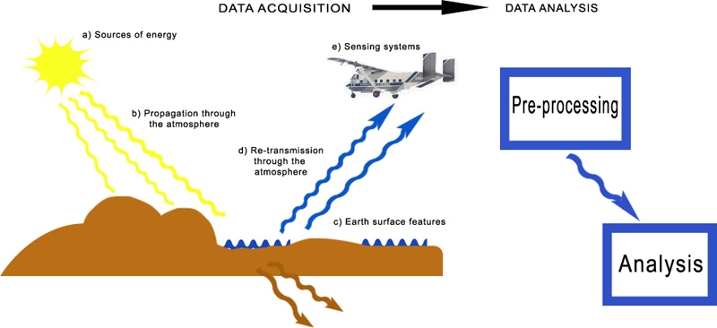
A review of the remote sensing process with a S/N perspective is a good place to start. The remote sensing process consists of:

1. the sun as a source of radiant energy,
2. transmission of solar radiation through the atmosphere,
3. interaction of the solar radiation with the surface,
4. transmission of reflected solar radiation back through the atmosphere towards the sensor,
5. interception of the radiation by the sensor, and
6. analysis.

The process is a system with input (solar energy) and output (information). Each component of the system modifies or adds to the signal. Thus, each component has its own modulation transfer function or MTF. Although MTF is most often associated with image/signal processing theory, the idea that the atmosphere, earth's surface, and the electronics modulate the information content of the energy flow through the system is the same. We can thus speak of an atmospheric MTF, a surface MTF, and an instrumentation system MTF. The modulation process induces a noise component to the signal that is sensed by the detector and made available to the analyst.

The quantity of radiant solar energy received by the earth is very stable over any given six-month period. Our concern with the sun from a S/N perspective concentrates on the effects of solar zenith and azimuth changes on the direction and size of shadows, and the amount of energy that reaches a particular surface. This is why airborne remote sensing data collection (including aerial photography) at optical wavelengths is usually limited to plus or minus 2 hours from solar noon. The geometry of illumination relative to viewing geometry modulates the signal. These issues fall under the realm of the bidirectional reflectance distribution function (BRDF).

The atmosphere modulates the incoming or downwelling radiant solar energy via scattering and absorption before the energy interacts with the earth surface. More haze translates to more diffuse radiation than direct beam solar radiation reaching the surface. From the S/N perspective, this means that shadows not be as dark.

The interaction of solar energy with earth surface materials can be viewed as a modulation. Multiple factors contribute to the modulation, especially for the case of plant canopies. One way to understand what factors are important to energy interactions is to examine inputs to radiative transfer (RT) models used to calculate reflectance from surfaces. Plant canopy RT models such as the SAIL model are especially helpful. Inputs include the foliage density expressed as leaf area index (LAI), leaf reflectance and transmittance, soil reflectance, information about leaf angles relative to vertical, and the amount of diffuse solar radiation relative to direct beam solar radiation (as per the atmospheric MTF above). This explains why spectral vegetation indices are sensitive to a variety of characteristics such as plant foliage density, leaf reflectance, percent vegetative ground cover, and soil brightness.

Solar energy is reflected back into the atmosphere following interaction with surface materials Once again, there is modulation of the signal as the energy is scattered and absorbed by atmospheric constituents. The result of the atmospheric modulation is the addition of the atmospheric signal as haze to the information from the surface interactions.

The sensor system with its optics, detectors, spectral discrimination system and electronics is a a form of transducer. A transducer converts one form of energy into another. Sensor systems convert radiant energy into electrical energy. Thus, the output of the sensor system is a voltage. The voltage is a function of all of the prior remote sensing system components and the electro-optical sensor system. The optical subsystem and the electrical subsystem both add noise to the sensing process, thus further modulating the information signal from the environment.

Note that the sensor platform (fixed wing aircraft or helicopter), also induces noise via attitudinal changes. Roll, pitch and yaw changes while scanning induce geometric distortions, and if extreme enough, BRDF noise.

The analysis of sensor output can also be thought of as an opportunity for signal modulation. Enhancements, data compression, transformations, etc. can induce noise that hinders the extraction of desired information.

The modulation of the energy by the sun, atmospheric, target, and electro-optical system can be thought of as the process by which noise is induced to the final output of the sensor that undergoes analysis. A radiometric measurement expressed as a pixel can be though of as a sum of the desired information signal and a noise signal.

So in effect, each step or element of the remote sensing process introduces noise to the signal. A common goal of electro-optical system engineering, data collection, system calibration, and data processing is to maintain employ techniques that produce a high fidelity system: tools that reproduce the input information faithfully, or accurately.

Disclaimer

Acknowledgements

III. A Primer on Imaging Theory: What to expect from imagery

Knowledge of the imaging process can help formulate reasonable expectations for airborne imagery. The imaging process is imperfect and thus produces an abstraction of reality. To the analyst this means that there will always be recognizable characteristics of the electro-optical imaging process present.

Imaging theory uses linear systems concepts. The mathematical representation of the imaging process uses a convolution function. A graphical representation of the imaging process as a convolution without equations is sufficient to illustrate this concept. The imaging system is represented by a function (illustrated here by a non-symmetric function). The environmental "target" can also be represented by a function (here a symmetric, binomial distribution). Note that the imaging system is not represented as a "perfect", symmetric function or as a square wave. The scanner system function is normalized from 0.0 to 1.0. A scanner function value of 1.0 would indicate that the system perfectly transmits the input information signal (from the environmental target) to its electronic output form (a digital number). A value close to 0.0 indicates that the scanner system does a poor job of transmitting the input signal. If imaging systems were entirely perfect they would be represented as square waves: 1.0 or perfect signal transmitters.

The process of scanning the target can be visualized as an integration of the two functions. The final result of this process is a third function with characteristics of both the scanner system and the environmental target. Given a system with a high S/N and thus high fidelity, the resulting output image (here represented as a function), would be a faithful or true representation of the environmental signal. Graphically, an output from a high fidelity system will be a function that looks very much like the input function. Note that if the input signal consists of the desired environmental signal (with its inherent noise), plus an atmospheric signal (more noise), the S/N going into the scanner is already be an issue. If the platform attitude is unstable, (adding more noise), and the scanning process adds its own noise, one can understand why S/N is a reasonable approach to airborne remote sensing.

What one can reasonably expect from imagery varies largely as a function of the system design. The Jet Propulsion Laboratory (JPL) Advanced Visible InfraRed Imaging Spectroradiometer (AVIRIS) is widely accepted to be state-of-the-art for airborne imaging devices available to the civilian environmental remote sensing community. With AVIRIS as the top-of-the-line and an analog video system as the other extreme, users of most airborne imaging systems can expect data quality that is somewhere between these two.

Silicon Detector Sensitivity Effects

Attention to silicon detector sensitivity is important when choosing spectral bands at the upper and lower limits of spectral sensitivity. A plot of the sensitivity of silicon by wavelength shows this graphically. Note the peak sensitivity of silicon in the visible wavelengths and the rapid fall-off of sensitivity for the UV and NIR. Decreased sensitivity translates to more noise. Unless a system is specifically configured to maximize S/N for the extreme UV and NIR, when specifying narrow bandwidth spectral channels, it is widely recommended that wavelengths below 500 nm and above 1000 nm be discarded. Scanners may be listed as being "sensitive" to wavelengths below 500 nm and above 1000 nm, however this does not always translate to good quality data. If data covering below 500 nm and above 1000 nm is needed, one can try broader spectral band widths to average out the noise.

Platform Nose Pitch Problems and Geometric Fidelity

A very difficult problem to diagnose is geometric distortion that occurs when the aircraft nose pitches downward while scanning. Airborne scanner systems use the scanning mechanism (electronic for push-broom systems or mirror sweep for whisk-broom systems) for the across-track image dimension and the forward motion of the aircraft for the along-track dimension of the image. If the aircraft nose pitches downward during the scanning process, the system continues to scan backwards off-nadir along track as the nose goes down. As the nose comes back up, the system is still scanning and re-scans off-nadir the same part of the landscape that was just scanned in the forward and backward directions. This is very difficult to identify visually, especially over crops. It is usually noticed if a ground feature appears in the imagery more than once.

Framing systems such as digital cameras are easier to geometrically rectify as every pixel of the image will have the same geometry at the time of acquisition. A rubber-sheet stretch usually does an acceptable correction for reasonably-level landscapes given suitable ground control tie points. Push-broom and whisk-broom scanning systems theoretically have a different solution for every pixel. Variations of roll, pitch and yaw in time affect each pixel as it is formed. Rubber-sheet stretches are typically more challenging to perform with such imagery. If the system is equipped with an Inertial Navigation System (INS) to measure and record platform roll, pitch and yaw periodically, first-order corrections for platform attitude changes can be automatically performed. Some additional corrections are still needed, however.

Disclaimer

Acknowledgements

IV. Simple Tools for Checking Image Data Quality

The imaging process is not perfect and noise is always present from the:

• Solar illumination
• Atmosphere
• Earth surface target interactions
• Imaging system (including platform)
• Analysis

A fundamental question that investigators must ask themselves following data collection and before image analysis is: Is the data worth analyzing? There are simple checks investigators can perform to assess data for an idea as to its fidelity. Keeping the S/N model in mind, the investigator must continually ask if the data "makes sense".

Step 1: Check the header for correct data collection conditions and settings. Some of the following information may not always be available. Is the imagery correct for:

• date
• time
• location
• units
• calibration file date
• GPS datum
• GIFOV
• platform airspeed
• platform altitude
• aircraft type and tail number
• pilot name
• instrument operator(s)

Operator notes, both written and verbal (via recordings of cabin intercom conversations via a tape recorder or audio track of a VCR) are also useful. Pay particular attention to notations and times of radio contact with other aircraft or air traffic control as radio transmission has been known to cause radio frequency (RF) interference of imagery.

Step 2: Make "quicklook" false color pictures using standard color infrared assignments: B,G,NIR bands. Briefly examine each spectral band in black and white. For hyperspectral data, a sampling of spectral bands across visible-blue, visible-green, visible-red, several near infrared, and several short wave infrared bands are suggested.

Look for:

• Indications that the general location of the coverage is correct such as known features of the landscape
  • clouds
  • cloud shadows?
  • Odd features?
  • Imaging characteristics?
  • Noise level?
• Do the features present seem reasonable given your knowledge of the landscape?
• Do any anomalies indicate possible problems with the system, calibration, or platform?
• Are there "blooms" or either dark or light/white areas that mask surface detail?
• Is there a gradient of light to dark or dark to light at one of the edges of the image?

These could indicate the need for additional calibration steps, or hardware problems.

Step 3: Assess the locational and cartographic/geometric fidelity of the imagery. Locational accuracy of imagery is easiest to determine given analyst knowledge of the landscape - look for familiar features and ask yourself if they appear as they should. Geometric rectification of imagery is easiest to ascertain if a GIS shape file is generated using surface-based differential GPS and then overlain on the imagery.

• Does the GPS record indicate the correct location was flown?
• Are landscape features positioned where they should be relative to each other?
• Are straight-line features such as roads, railroad tracks, etc., showing up as straight lines?
• Do curved features have their characteristic gradual or sharp curvature?
• Does the image appear to have been taken from a level platform with minimal roll, pitch, and yaw?

If the system is equipped with an Inertial Navigation System (INS), roll, pitch and yaw are measured and logged every couple of scan lines. The INS data coupled with the GPS data permits a very good first order geometric rectification. However, there will still be some minor locational errors of no more than 2-3 pixels at high spatial resolution (1-4 m)

Step 4: Print histograms of each spectral band image. Histograms provide a snapshot of radiometric values for an entire spectral image. Examine the histograms for:

• shapes relative to scene contents?
• shapes relative to each band?
• continuous or with noticeable dropouts?
• units consistent?
• range of values?

Are the histogram distributions univariate, bivariate, normally distributed, skewed, continuous? Are the distributions continuous or are there ranges of values missing that indicate a hardware problem? Are the values high or low according to what one would expect from the spectral band being examined? Are the amplitudes consistent with the units?

Given an image dominated by plant canopies, the histogram for VIS-red should be show the majority of the values to be fairly low. The opposite would be true for NIR values. Very low NIR values should be present if there are clear water bodies present. Conversely, the presence of clouds would show up as high values across all spectral bands.

Do these histograms seem reasonable based on what you already know about the landscape and the conditions under which the data was collected?

Step 5: Extract pixel values across all spectral bands for familiar features and plot the signatures. A major tenet of remote sensing is that information about a target on the earth's surface is available from any altitude. Look at the signatures and assess whether or not they look like something familiar from your knowledge of the literature or from ground-based measurements using field-portable instrumentation. Suggested features are:

• dense vegetation - crops, trees, etc.
• turf grass
• low percent cover vegetation with some soil showing through
• bare soil
• blacktop roadways
• deep waterbodies
• concrete surfaces

Plant canopies should have the familiar plant canopy signature. Bare soil should have the characteristic "ramp-like" signature. Compare vegetation signatures -crops versus dense tree canopies for example. The chlorophyll absorption well in the red and the NIR plateau should be especially useful. Blacktop surfaces should appear very low in reflectance across VIS and NIR wavelengths. The low reflectance targets should be useful as places where noise problems will occur. The 3% - 5% low reflectance of full cover plant canopies is especially tough for remote sensing systems to handle.

Do these signatures seem reasonable based on what you already know?

Disclaimer

Acknowledgements

V. Choice of Spectral Bands

There is a rich heritage of knowledge from over 20 years of electro-optical remote sensing research. Draw upon this and use it as a starting point when approaching a data set. Fundamental relationships between specific spectral bands and plants and soils are well documented. Look at the relationships between red and NIR and various plant characteristics. Then try NDVI. When specifying spectral bands for analysis, channels with band centers close to the band centers of Landsat ETM+ are a good choice:

Band Number	Spectral Range (nm)
1	450 to 515
2	525 to 605
3	630 to 690
4	750 to 900
5	1550 to 1750
6	1040 to 1250
7	2090 to 2350
Panchromatic	520 to 900

Terra satellite MODIS or the EO-1 satellite Hyperion instrument spectral band configurations are also reasonable choices.

Note the potential pitfalls of specifying narrow spectral bandwidths below 500 nm and above 1000 nm as explained in the section on Silicon Detector Sensitivity. Another factor to consider is the bandwidth of the system. The AISA, like many low-cost airborne scanner systems are "band-width limited", meaning that only so much data can be handled at a time. This forces users to balance the need for many spectral bands with the need for high spatial resolution ground instantaneous field of view (GIFOV). As the GIFOV increases, the number of available spectral bands will decrease.

HYPErspectral or Multispectral?

Despite over 20 years of electro-optical multispectral and hyperspectral image research, NDVI is still the most widely used approach for analysis. Hyperspectral exploitation has lagged, presumably because of the lack of widespread data availability to the remote sensing research community, and because of a lack of pressing scientific justification. One can better understand this by addressing why the HIRES instrument was deleted from the NASA EOS/Terra satellite. Thus, spectral vegetation index (SVI) approaches are still very appropriate.

Land cover classification accuracies have been shown to improve from the use of hyperspectral imagery. Recent work on the value of improved sensitivity of narrow spectral bandwidths to vegetation characteristics when using SVI analysis is further evidence of the potential of hyperspectral imaging. Red Edge analysis also relies on hyperspectral data as does spectral unmixing.

Disclaimer

Acknowledgements

VI. Final Thoughts and Suggestions

Collecting, processing and analyzing airborne remotely sensed data is more difficult than working with data from field portable radiometric instrumentation or satellite data. The platform characteristics (roll, pitch, yaw, airspeed), altitude of data collection (in the atmospheric column versus above or below it), calibration issues (handled by someone else with satellite data or is non-imaging as with field instruments), choices and trade-offs between spatial, spectral, and radiometric information domains, and its intermediate level of technology create challenges for the user.

One suggestion to investigators using airborne imagery that has always proved to be a useful learning experience is to take a ride in a small aircraft or a helicopter at the altitude of most data collection over an area of interest. Take a 35 mm camera and a pair of binoculars. Try and keep the binoculars on a specific feature of the landscape and note the motions of the aircraft. Note ground and sky conditions such as soil moisture, surface winds, atmospheric haze, etc.

Keep the concept of S/N in mind when looking at airborne imagery. You as the user and/or analyst must ultimately decide the answer to one key question: Does the data have an acceptable S/N to warrants its use?

Disclaimer

Acknowledgements

VII. References and Resources

The following resources have proven useful and are provided with notes so that readers will more easily find specific information.

Web Sites

John Bolton's virtual Center for Airborne Remote Sensing Technology Development. An excellent source of links. There is also a very good, brief explanation of airborne sensor calibration issues. http://CARSTAD.gsfc.nasa.gov

Satellites and Systems

NASA Earth Observer - 1 new technology demonstrator satellite. http://eo1.gsfc.nasa.gov/

NASA Landsat satellite. http://landsat.usgs.gov

NASA Terra satellite MODIS instrument. http://modis-land.gsfc.nasa.gov/

3Di, LLC, airborne data provider and vendor of AISA systems. http://www.3Dicorp.com/

Specim - the Finnish company that builds AISA. http://www.specim.fi/index.html Data Accuracy Standards

Federal Geographic Data Committee http://www.fgdc.gov/

American Society for Photogrammetry & Remote Sensing 1995 Draft Standards for Aerial Photography http://www.asprs.org/resources.html

American Society for Photogrammetry & Remote Sensing Digital Imagery Guideline Committee http://www.asprs.org/society.html

Books

Instrumentation, Radiometry and Calibration

1. McCluney, Ross, 1994. Introduction to Radiometry and Photometry. Boston, Artech House, 402 pp. A useful resource on the basics of radiometric measurement. Notable for its explanations of geometry, units, basics of radiation measurement, optics. A good, readable introduction to the concepts.

2. Schott, John R., 1997. Remote Sensing: The Image Chain Approach. New York, Oxford Univ. Press. 394 pp. An advanced remote sensing textbook. Many elements are updates on topics covered by the book by Slater (below).

3. Slater, P. N., 1980. Remote Sensing: Optics and Optical Systems, Reading, Addison-Wesley Publ. Co., 575 pp. Classic book covering the technical details of remote sensing from radiometry, interactions of solar radiation with the atmosphere and the earth's surface, optics, units, spectroradiometric calibration, BRDF, etc. Notable for its description of the Suits vegetation canopy reflectance model (basis for the SAIL model) starting on p 256, MTF in Appendix 1.

4. Smith, G. M. and P.J. Curran, 2000. "Methods for Estimating Image Signal-to-Noise Ration (SNR)", Chapt. 5 in Atkinson, P.M. and N.J. Tate, Advances in Remote Sensing and GIS Analysis, Chichester, John Wiley & Sons, 273 pp.
A summary of methods used to calculate imaging system S/N from imagery.

Radiative Interactions with the Atmosphere and Earth Surface Features

1. Asrar, G., (ed.), Theory and Applications of Optical Remote Sensing, 1989. New York, John Wiley & Sons, Inc., 734 pp.
A useful reference on many remote sensing science topics. The chapter on The Atmospheric Effect on Remote Sensing and its Correction (p. 336) is an especially good introduction to the topic.

Imaging Theory and Image Processing

1. Castleman, Kenneth R., Digital Image Processing. 1982, Englewood Cliffs, Prentice-Hall, Inc.429 pp. Introductory image processing text for computer science courses on the topic. The section on imaging theory describing the convolution process on p.145 is especially helpful.

2. Jensen, John R., Introductory Digital Image Processing: A Remote Sensing Perspective. 2nd Edition, 1996, Upper Saddle River, Prentice-Hall, Inc. 318 pp. Introductory image processing text for environmental remote sensing courses. The chapter on Image Preprocessing and a part of the Image Enhancement chapter on Special Transformations are especially useful.

3. Russ, John C., The Image Processing Handbook, 4th Edition, 2002. Boca Raton, CRC Press Inc., 732 pp. A useful, general reference covering all aspects of digital image processing and digital imaging. Easy to read.

Journal Articles and Proceedings Papers

Moran, M.S., T.R. Clarke, J. Qi, E.M. Barnes and P.J. Pinter, Jr., 1997. Videography and Color Photography in Resource Assessment. Practical techniques for convesion of airborne imagery to reflectances. Proc. Of 16th Biennial Workshop on Videography and Color Photography in Resource Assessment, Weslaco, TX April 29-May 1, 1997. American Society for Photogrammetry and Remote Sensing and the USDA Subtropical Agricultural Research Laboratory.

Home

Disclaimer

Acknowledgements

Disclaimer

Acknowledgements