BTS Home > Publications > Journal of Transportation and Statistics > Volume 3 Number 3

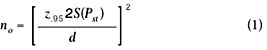
Vehicle Speed Considerations in Traffic Management: Development of a New Speed Monitoring Program

Darren L. Jorgenson
Ernst and Young

Matthew G. Karlaftis*
National Technical University of Athens

Kumares C. Sinha
Purdue University

Abstract

Since the passage of the National Maximum Speed Limit (NMSL) of 55 miles per hour (mph) in 1974 through its repeal in 1995, the federal government has mandated speed monitoring programs. The speed monitoring program was primarily intended to provide reliable data for inclusion in states’ annual certification for Federal Aid Highway Projects. The repeal of the NMSL in 1995 not only authorized states to set their own speed limits but also allowed them to develop their own speed monitoring programs. This paper develops a seven-step framework for a speed monitoring program tailored to meet the needs of individual agencies using speed monitoring data at the state level. The proposed speed monitoring plan distributes speed monitoring stations to highway classes according to three primary criteria: spatial distribution, crash distribution, and daily vehicle-miles traveled (DVMT) distribution. The proposed plan is also compared with the existing speed monitoring program.

Introduction

The objective behind the design of any engineered public facility is to satisfy the demand for service in the safest and most efficient manner. As such, speed is one of the traveler’s foremost concerns when selecting alternate routes or transportation modes. Directly related to its speed, convenience and economy largely determine the value of a transportation facility in carrying people and goods.

At the same time, speed relates to travel safety. The National Crash Severity Study (NCSS), an investigation of approximately 10,000 crashes from 1977 to 1979, revealed that the possibility of fatality increases dramatically as the change in velocity during the collision increases (Flora 1982). This study showed that a driver crashing with a change in velocity of 50 miles per hour (mph) is twice as likely to be killed as one crashing with a change in velocity of 40 mph.

Vehicle speed contributes to crash probability, and an exceptionally important factor is the variability in speed on the same segment of highway. Speed variance, a measure of the relative distribution of travel speeds on a roadway, relates to crash frequency in that a greater variance in speed between vehicles correlates with a greater frequency of crashes, especially crashes involving two or more vehicles (Garber 1991). A wider variability in speed increases the frequency of motorists passing one another, thereby increasing opportunities for multi-vehicle crashes. Because vehicles traveling the same speed in the same direction do not overtake one another, as long as the same speed is maintained, they cannot collide. There have been several notable and exhaustive literature reviews in the area of speeding and crash probabilities, covering both the U.S. and abroad, worth consulting. See Transportation Research Board (TRB) (1998).

An important determinant of traffic safety is effective speed enforcement. While enforcement techniques have changed over the years, the principal reasons for controlling vehicle speeds, protection of life and property against the hazards of highway travel and efficient use of street and highway systems, have not. Speed monitoring data allow agencies to set up enforcement strategies, which will reduce speeds and, consequently, increase safety. Vaa (1997) conducted a field experiment in which a 35-kilometer stretch of road was subjected to an increase in police enforcement. Speed was measured in 60 and 80 kilometer per hour (km/h) speed limit zones before, during, and after enforcement withdrawal and compared with another stretch of road. Average speeds were reduced in both speed limit zones for all times of day. For some time intervals, the average speed and the percentage of speeding drivers were reduced for several weeks after the period of enforcement, demonstrating a time-halo effect1 of eight weeks.

The present study discusses the necessary steps in developing a speed monitoring program and uses data from the state of Indiana to adjust the program to the needs of the state. Several factors warrant the present study. First, the existing speed monitoring program is designed to meet federal requirements and does not necessarily address the particular needs of state agencies. Second, speed monitoring stations are distributed to highway classes based solely on daily vehicle-miles traveled (DVMT), while states may find it appropriate to use additional criteria for monitoring station distribution. Finally, the existing program does not account for geographic gaps between stations where no monitoring occurs. The remainder of this paper is organized as follows: the second section discusses the existing, federally mandated, speed monitoring program and the current speed monitoring practices in various states. The third section identifies the speed monitoring needs for the state of Indiana and provides an overall strategic framework for the proposed speed monitoring plan. The fourth section presents the proposed speed monitoring program along with a comparison of the existing program, and the last section offers some concluding remarks and recommendations.

Background

In 1973, Congress established a National Maximum Speed Limit (NMSL) of 55 mph, initially as a temporary energy conservation measure. In 1974, Congress made the national maximum speed limit permanent. The Federal Aid Amendments of 1974 made annual state enforcement certification a prerequisite for approval of federal aid highway projects. Summary data from state speed monitoring programs were a part of these annual certifications. The “Procedural Guide for Speed Monitoring,” issued September 1975, provided the first federal guidelines for speed monitoring (USDOT FHWA 1975). The original speed monitoring procedures were designed to collect data and produce statistics for each of five highway types in a state on level, tangent highway sections under “free-flow” conditions. The methods for calculating statewide statistics, however, varied among the states, making the value of state-to-state comparisons questionable.

Slowly declining compliance with the 55-mph speed limit and increasing accident and fatality rates prompted the U.S. Department of Transportation (USDOT) to recommend, and Congress to approve, significant changes in the speed limit legislation in 1978 (USDOT FHWA 1978). The Highway Safety Act of 1978 provided for both withholding of federal aid highway funds and awarding incentive grants based on annually submitted speed compliance data. An estimate of the percentage of motor vehicles exceeding 55 mph became the major reporting requirement. Further changes to the speed monitoring program included that “free-flow” would no longer be the only condition monitored. Speed statistics must be representative of all travel; thus, all vehicles passing a monitoring station during the observation period had to be measured. Furthermore, speeds could be monitored on other than level, tangent sections of highway.

In 1980, further changes were made when the "Speed Monitoring Program Procedural Manual" (SMPPM) (USDOT FHWA 1980) was issued. Some of the most important points include the following: 1) sampling sessions were to be 24 hours long in order to account for varying daily traffic conditions affecting speeds; 2) highways were stratified into 6 categories based on Federal Highway Administration (FHWA) classifications instead of the 5 categories based on geometry as they were previously defined; 3) sampling sessions were allocated among highway categories based on the statewide DVMT, subject to the 55-mph speed limit in each highway category; 4) within a category, locations were picked using simple random sampling with probabilities proportional to mileage, commonly known as probability sampling; and 5) the target sampling accuracy of the annual statewide value of percentage of DVMT over 55 mph was 2.0% at a 95% confidence level. The number of sampling locations was established as the greater of the numbers needed to meet the target sampling accuracy and the DVMT subject to the 55-mph limit divided by two million.

On April 2, 1987, the Federal Aid Highway Act of 1987 gave “the states the authority to increase, without the loss of Federal Aid-funds, the maximum speed limit to no more than 65 mph…on Interstate Systems located outside an urbanized area of 50,000 (population) or more.” Also, “Any state choosing to increase the speed limit from 55 mph…will have to adjust the speed sampling and analysis plan in effect for the fiscal year in which the limit is raised.” A memorandum the FHWA distributed advised states choosing to increase the speed limit on eligible sections of rural interstate highways that DVMT represented by mileage in areas where the speed limit had been raised above 55 mph would not figure into the calculation of 55-mph-speed-limit compliance statistics for fiscal year (FY) 1987. In essence, DVMT factors would be adjusted to exclude all rural interstate locations where the maximum speed limit had been reposted to 65 mph. Even though a process of redistribution of DVMT weighting factors would exclude the requirement of monitoring and reporting statistics for rural interstate highways, the same number of locations would continue to be distributed among the (remaining) functional groupings in the same proportion as before.

In December of 1991, the Intermodal Surface Transportation Efficiency Act (ISTEA) was signed into law. FHWA and the National Highway Traffic Safety Administration (NHTSA) subsequently published modifications governing the National Maximum Speed Limit (NMSL). The revised procedures established speed-limit compliance requirements on both 55-mph and 65-mph roads. This statute assigned greater weight for speed limit violations in proportion to the degree motor vehicles exceed the speed limit. Additionally, the ISTEA compliance formula was tied more closely to the relative risk of fatality and to a measure of crash severity. On November 28, 1995, new federal legislation repealed the National Maximum Speed Limits, ending two decades of mandates. Effective December 8, 1995, states were again authorized to set their own speed limits and speed monitoring policies.

Jorgenson (1998) conducted a survey of the current speed monitoring practices from May of 1997 through July of 1998 in all 50 states. Since the repeal of the NMSL, 30 states have elected to change their speed monitoring programs. Of those 30 states, 8 states currently have more monitoring stations than previously mandated by the FHWA. Of the 22 states that reduced the number of monitoring stations, 11 dropped the speed monitoring program altogether (table 1).

Identification of Speed Monitoring Needs

After the repeal of the NMSL, the most important question for the state of Indiana became if the speed monitoring program should be continued. A simple questionnaire was distributed to parties interested in speed monitoring: the Indiana State Police, the Indiana Department of Transportation (INDOT) Planning Division, INDOT Roadway Management Division, FHWA safety engineers, and others. As table 2 shows, the respondents almost unanimously supported a speed management program. The respondents considered it important to continue speed monitoring following the repeal of the NMSL in order to devise suitable enforcement measures, ensure safety on the state road network, provide speed information to various public and private agencies, and have reliable data readily available for design, operational, and research needs.

Once the need for and desire to participate in a new speed monitoring program was established, the second question became the criteria by which monitoring sites were to be distributed among highway classes. After discussions with the participants in the preliminary study, three considerations for site allocation were chosen: 1) spatial distribution, 2) relative DVMT distribution, and 3) relative crash distribution. The crash distribution criterion was further broken down into four types of crashes: all crashes, all fatal crashes, speed-related crashes, and fatal speed-related crashes. The six highway classes chosen were rural interstates, urban interstates, rural U.S. roads, urban U.S. roads, rural state roads, and urban state roads. Sites have historically been distributed by functional highway class. In the proposed plan, two factors influenced the decision to consider a different highway classification scheme. First, all supporting data used in the present study, such as vehicle-miles traveled and crash data, were available for the new classification scheme. This consistency allows any agency using speed data to easily investigate causal relationships. Second, there was evidence of a statistically significant difference in the mean speed of these highway classes (Jorgenson 1998).

We used a Delphi study to ensure that the allocation of speed monitoring stations be consistent with the requirements of those using the resulting data by ranking and rating the site distribution criteria. The Delphi process allows a group with varying opinions to come to a consensus. In the present study, the objective was to rank and rate speed-monitoring station distribution criteria. The Delphi process replaces direct confrontation and debate with a carefully planned, orderly program of sequential discussions, carried out through an iterative survey (Dalkey et al. 1969). Typically, a presentation of observed, expert concurrence in a given application area where none existed previously results (Sackman 1974). In this portion of the survey, participants were first asked to allocate 100 points among the three distribution criteria. The higher the number, the more important that criterion was deemed. For the next step, participants allocated 100 points among the four crash categories. Again, the higher the number, the more important that crash type was deemed.

Table 3 provides the results of the Delphi process. Following the first round, DVMT was the highest rated distribution criterion with 36 points. Crash distribution was second with 33 points, and spatial distribution was third with an allocation of 31 points. The crash results showed speed-related crashes to be the most important crash distribution criterion with an average 29.3 points. Fatal speed crashes followed with an average of 28.6 points. All crashes came in third with an average of 24.7 points, and all fatal crashes was fourth with an average of 20.0 points. In the second round, the order of importance for both the distribution criteria and crash types changed. As table 2 shows, DVMT continued to be the most important distribution criterion with an average 34.8 points. This was closely followed by spatial distribution, up from third place in the first round with an average value of 34.2. Crash distribution was last with a mean value of 31.0. While this result may seem counterintuitive to some in that crash distribution would be deemed the least important, it demonstrates the power of the Delphi approach: criteria importance is based on collective results rather than on single opinions.

The order of importance for crash types also changed. Speed-related crashes remained in first place with an average 28.8 points. All crashes moved up from third to second with an average 27.9. Fatal speed crashes dropped from second to third place with an average of 24.3. Finally, all fatal crashes remained fourth with an average of 19.0. Because the Delphi process deliberately manipulates responses toward minimum dispersion of opinion in the name of consensus (Martino 1972), there is no advantage to continuing beyond two rounds (Dalkey 1970). Therefore, the survey stopped at that point. Having identified both the desire and need for a speed monitoring program and the criteria to develop it, we then developed the basic procedure to define the number, location, and monitoring time of the new program.

Design of the Speed Monitoring Plan

In order to maintain, as much as possible, compatibility with the data collected under the FHWA program, the new program’s design, follows the statistical requirement of a 2.0 mph maximum error of estimate, with 95% confidence, as used in the federal program (USDOT 1992). This requirement determined the following seven core components of the proposed program: 1) the number of monitoring sessions per year, 2) duration of monitoring period for individual sampling sessions, 3) monitoring speed by direction of travel, 4) monitoring speed by vehicle length, 5) the minimum number of statewide sampling locations, 6) monitoring station site distribution, and 7) selection of monitoring locations. Finally, the proposed program has speed monitoring stations allocated by highway class based on the distribution criteria discussed in the previous section. We also discuss here a procedure to help determine locations of monitoring sites utilizing existing speed monitoring, weigh-in-motion (WIM), and automated traffic recording (ATR) stations.

Number of Monitoring Sessions per Year

The federally developed monitoring program collects speed data every quarter (USDOT 1992). However, while it is well documented that traffic volume varies by time of year (McShane and Roess 1990), the variation in mean speed by time of year may not be significant. The present study examines the need for quarterly speed monitoring. The existence of a significant difference in mean speed by quarters and of a significant difference between each quarterly speed distribution could determine the necessity of quarterly speed monitoring.

A three-stage, nested factorial design (Montgomery 1997) serves as the statistical model used to analyze the number of monitoring sessions per year. A nested, factorial design was chosen because levels of one factor are similar but not identical for different levels of another factor. This means, for example, that highway class one in district one of year one is similar to, but not identical to, highway class one in district one of year two. Therefore, highway class is nested under district one in year one. This analysis used the historical 1983 through 1997 speed monitoring data collected in Indiana. The database covered 15 years, 4 annual quarters, 6 districts, and 6 highway classes. The total of 320 stations represented different monitoring locations used over the 15-year period. Appendix one shows the model for the three-staged, nested factorial design used in this experiment representing the main effects and their associated interactions. The model was estimated with SAS (1998) in order to test for significant main and interaction effects. The Student-Newman-Keuls (SNK) multiple range test was used on all main effect means (Everitt 1992). The SNK method compares all pairs of treatment means in an effort to discern which means differ.

The experiments of interest in this analysis were variation by quarter, variation by quarter by class, variation by quarter by district, and variation by quarter by district by class. Table 4 shows the significance probabilities associated with each main effect and interaction this analysis used. From this table we can determine the significance of the relevant main effects and their interactions. The probability associated with the main effect of quarter, denoted by γ _m (0.9054), indicates that no significant difference in mean speed existed between quarters. Mean speeds stratified by quarter, presented in table 5, demonstrate that the mean speed only varied from 58.8 mph in quarter 1 to 58.9 mph in quarter 4, further showing that mean speed was not significantly different by quarter. The probability associated with the quarter by class interaction effect, denoted by χγ _km (0.8790), indicates that mean speed is not significantly different by quarter and highway class. The probability associated with the quarter by district interaction effect, denoted by βγ _jm (0.5505), indicates that mean speed is not significantly different by quarter and district. The probability associated with the quarter by district by class interaction effect, denoted by a αβχγ _ijkm (0.6947), indicates that mean speed is not significantly different by quarter within each highway class and district. Nevertheless, it should be noted that there is preliminary evidence that although the mean speed was found not to be different by quarter, the speed distributions may be. This hypothesis was tested using Fisher’s c ²-test (Jorgenson 1998). Consequently, it may be desirable to continue to monitor speed every quarter.

Duration of Monitoring Period for Individual Sampling Sessions

Under the original FHWA program, a 24-hour monitoring period was selected for the following reasons. First, it accounted for the varying traffic conditions affecting speeds within a day. Second, the within-cluster (daily) variation would not allow for a reduction in the number of locations required even if much longer periods were used. The 24-hour monitoring period minimized cost in terms of the combination of sampling locations required and the need for equipment. For the proposed program, the Indiana State Police wanted to test whether day of week was a significant factor in determining mean speed. If so, it would be necessary to monitor speeds for a longer period, thus the need for this analysis. With a two-stage, nested factorial mixed effects model with data from 27 WIM stations distributed throughout the state, it was concluded that, at the 95% level of significance, the effect of day on mean speed was not a significant factor in explaining the variation in mean speeds in Indiana; thus, the future program should continue to monitor speeds 24 hours a day.

Monitoring Speed by Direction of Travel

The survey of state-wide speed monitoring practices revealed that half of the states that continue to monitor speeds do so in both directions of travel. Consequently, INDOT wanted to see if it was necessary for Indiana to measure speed by direction. Also, the Indiana State Police felt speed by direction could be important for enforcement purposes. A two-stage, nested factorial mixed effects model determined at the 99% level of significance that mean speeds were different by direction of travel. Based on this finding, speed should be monitored for each travel direction, particularly for divided highways.

Monitoring Speed by Vehicle Length

Since trucks are much heavier and have slower acceleration and deceleration rates than passenger vehicles, there is an increased potential for severity in cases of crashes between trucks and smaller vehicles. Higher speeds add to the severity of these crashes. At the same time, speed variance increases when trucks travel at a different speed than other vehicles. In Indiana, the speed limit for trucks on rural interstates is 60 mph, while for passenger vehicles it is 65 mph. Representatives from Indiana State Police, INDOT, and the Department of Revenue requested that an analysis determine if a difference existed in mean vehicle speed based on vehicle length, not only on rural interstates but also on other roads. A two-stage, nested factorial mixed effects model was estimated with station nested under highway class. Station is nested under highway class because different levels of station are similar but not identical for different levels of highway class. As the federal program suggested, speed by vehicle class was not monitored. A special data collection effort was made during the four quarters of 1997 to record speed data separately for trucks at randomly selected existing monitoring stations. Three vehicle classes were considered. Class 1 consisted of passenger cars 20 feet long or less; class 2, medium sized trucks between 21 and 40 feet long; and class 3, large trucks 40 feet long or greater.

Of interest in this experiment was whether vehicle class and the interaction between highway class and vehicle class were significant. Results show that highway class, vehicle length, and the interaction between highway class and vehicle length were all significant with probability (Pr > F ) values of 0.0001. Because Indiana currently employs differential speed limits on rural interstates, the interaction between highway class and vehicle class could be significant. It was found that mean speeds for the three vehicle classes considered were significantly different from each other. Passenger cars had a mean speed of 60.2 mph; single unit trucks and buses had a mean speed of 58.2 mph, and combination trucks had a mean speed of 59.4 mph. The results are somewhat surprising because one would expect single unit trucks to travel at a higher speed than combination trucks.

Number of Statewide Monitoring Stations

Two concepts were used to determine the number of statewide monitoring stations: reliability of statistical estimates and coverage of population sampled (Miller et al. 1990). In the FHWA program, the standard statistical requirements for determining sample size depend on the statewide standard deviation of the percentage of vehicles exceeding the posted speed limit rather than on mileage or vehicle-miles traveled (USDOT 1992). Since this figure would be similar in most states, the resulting sample sizes would be nearly the same, with the exceptions of very small states. This meant that, statistically, the sizes of the speed populations of different states had very little influence on the sample sizes required for estimation. Having nearly equal samples for the different states did not provide data representative of the widely varying travel characteristics found among the states. The concept of "coverage of population sampled" instead provided balance to the work load among the states and a margin of increased accuracy for the larger states with larger mileages and DVMT.

The FHWA program determined the minimum sample size needed for a state under each of the two concepts and then selected the larger of the two numbers as the statewide minimum sample size. In this manner, the reliability requirement can always be met, and the sample size can be sensitive to the varying amounts of travel in the states. The present study adopted the FHWA approach in determining the total number of stations in the proposed program. To determine the number of locations required for the desired precision, a preliminary estimate of the standard deviation was estimated. The present study used the default value for this parameter, set by the FHWA at 7.0%, to determine the number of stations required. The formula to calculate the number of monitoring stations follows.

Equation (1):

where
n_o = sample size,
z.95 = value of the normal distribution based on a one-sided 95% confidence interval,
S (Pst ) = standard deviation of the percentage of vehicles exceeding the posted speed limit,
d = precision level required (2.0 mph).

For Indiana, the number of sampling segments required by the reliability of statistical estimates criterion was 38.

The coverage concept was designed to allocate locations based on the amount of travel, DVMT, subject to the posted speed limit in the state. This concept served various purposes: 1) to provide a balanced sample size; 2) to compensate for the additional variation possibly present due to larger volume or larger mileage; and 3) to account for the potential variation in speed enforcement activities of different police departments, districts, or jurisdictions within a state. With DVMT data from the 1997 Highway and Pavement Management System (HPMS) (USDOT 1995) database, the number of monitoring stations required for Indiana under the coverage concept is 26 (Jorgenson 1998). Therefore, the greater of the reliability criterion and the coverage criterion require 38 stations in the proposed program.

Monitoring Station Site Distribution

Concept

With the statewide number of necessary speed monitoring stations determined, the next step was to distribute them by highway class. As mentioned in the previous section, the three distribution criteria adopted in the present study are spatial distribution, DVMT distribution, and crash distribution. The crash distribution criterion was further broken into four crash types: all crashes, all fatal crashes, speed related crashes, and fatal speed related crashes. The expected site distributions were first computed for each criterion and crash type. The individual distributions were then combined into a composite distribution based on the individual criterion’s importance.

Spatial Distribution

The procedure used to distribute the speed monitoring stations by highway class according to the spatial criterion considered the six INDOT districts as separate geographical areas. The HPMS database served to calculate the number of lane-miles in each highway class for each district, giving the percentage of lane-miles by highway class by district. This percentage was then multiplied by the total number of stations, yielding the number of stations by highway class by district. The number of sites in each highway class was then summed over the district, giving the expected number of stations in each highway class for the state, as shown in table 6.

DVMT Distribution

To determine site distribution based on the DVMT criterion, the HPMS database was used to compute DVMT for each highway class. The DVMT for each highway class was then divided by the total DVMT subject to the 55-mph or greater speed limit, giving the percentage of DVMT for each highway class. That percentage was then multiplied by the total number of stations, giving the expected number of stations by highway class for the DVMT criterion. These calculations are shown in table 7.

Crash Distribution

To allocate stations according to crash criteria, an average crash distribution was computed for each of the four crash types. The 1991–1995 crash data from the Indiana State Police Crash Information System Crash Master Files is a database containing records on all reported crashes in Indiana. Table 8 shows the average crash distributions for all crashes; this process was repeated for all crash types. Once the average crash distribution for each crash type and for each highway class was computed, the percentage value was multiplied by the total number of stations, giving the expected number of stations by highway class for each crash criterion. This procedure was repeated for each of the four crash types, and the results for all crashes are shown in table 9.

Composite Site Distribution

After obtaining six separate site distributions schemes, we then combined them into a composite distribution. The importance ratings provided by the Delphi study played a role at this stage. A weighted average site distribution scheme was devised by multiplying the associated weights with the respective site distributions and summing them over each highway class. The goal was to have a composite site distribution that statistically satisfied each site distribution criterion: the proportion of sites in each highway class for each distribution criterion should be equal to the proportion of sites in each highway class for the composite distribution. Because it would be almost impossible to find a composite site distribution that statistically satisfied all three distribution criteria, the present study attempted to satisfy the two most important site distribution criteria, DVMT and spatial distribution.

In order to obtain a composite site distribution, monitoring stations were allocated to highway classes, making the composite distribution statistically close to both the DVMT and spatial distribution. The proposed site distribution has 13 stations in rural interstates, 10 in urban interstates, 7 in rural U.S. roads, 2 in urban U.S. roads, 4 in rural state roads, and 2 in urban state roads.

Selection of Monitoring Station Location

The proposed program makes maximum use of the existing speed monitoring, WIM, and ATR stations without affecting the statistical reliability of the proposed monitoring plan. The three options considered for this purpose vary by the level of use of existing stations: minor, moderate, and major change.

The first option, minor change, uses existing stations if they are in the same district and highway class of the proposed station. In this option, existing stations receive priority in the site selection process. If a certain highway class in an existing station is not available, a new site is randomly selected. Cost savings is the benefit of this method because very few new stations need to be installed. The main drawback is the reduction in randomness of the site selection process. To select the monitoring location for minor change, an iterative procedure helps allocate sites to highway classes within districts according to a range of plus or minus one of the recommended number of sites, based on the number of sites available. The recommended number of stations was computed by taking the percentage of lane-miles in a given highway class for a given district and multiplying that number by the total number of stations in that highway class. This procedure ensures that sites are distributed evenly throughout the state and minimizes the difference between the actual and recommended stations per district and highway class.

The second option, moderate change, also utilizes existing stations but in a different manner. The stations are first randomly selected. Then, existing stations are chosen if they match the characteristics of the randomly selected stations (DVMT, number of lanes, location, preferably the same continuous highway, and so forth). This method has a moderate cost and degree of randomness.

The third option, major change, relies totally on random selection of sites. The benefit of this alternative is that sample segments are completely random. The drawback is the high cost associated with installing new stations. Moderate and minor change have the same number of stations in each district and highway class; the difference between the two methods is in how the highway segments for monitoring stations are selected. To allocate the monitoring locations for moderate and major change, a procedure similar to the iterative one used in minor change was followed, except that there was no constraint requiring the use of available stations. For moderate change, the randomly selected stations were substituted for existing stations, when feasible. For major change, no such substitution took place. For this reason, the actual locations of individual monitoring stations are different under moderate and major changes, even if the distribution of stations remains the same.

Based on the minor change option, 38 existing stations would be used in the monitoring program. With the moderate change option, 22 existing and 16 new stations would be used. Based on the major change option, of the 38 randomly selected segments, 37 would be new stations and only 1 would be an existing station. It was a coincidence that this existing station was randomly selected. Because the primary objective of the study was to utilize as many existing speed monitoring stations as possible, the present study uses the minor change option of 38 existing speed monitoring stations.

Comparison of Proposed with Existing Site Layout

A comparison of the proposed site layout with the existing site layout indicated if the proposed site layout would be an improvement over the existing program. The underlying assumption in the present study’s sample size calculation was that the relative precision of the estimates would not exceed 2.0 mph. The relative precision can be calculated using the sample size and standard deviation of the percentage of vehicles exceeding the posted speed limit. The calculation of relative precision for the existing program used data from existing sites. For the proposed program, the standard deviation of the percentage of vehicles exceeding the posted speed limit had to be estimated using historical data.

Table 10 shows the proposed and existing site layouts with the expected number of stations for each of the site distribution criteria. The probability-values (p) under the expected values indicate the probability that the given site distribution will be similar to the distribution occurring from the listed site distribution criteria. A low p-value (<.05) indicates significant evidence of dissimilarity between the distributions. From this table, we can see that the proposed distribution is similar to the distribution yielded by the DVMT and spatial criteria. This means that the proposed distribution is not significantly different from those distributions based on the DVMT and spatial criteria. The existing distribution, however, is only similar to the distribution yielded by the crash criterion. In other words, the proposed station distribution satisfies two of the three distribution criteria, while the existing site distribution only satisfies one distributional criterion.

Conclusions

The present research reviews the federal speed monitoring program from its inception in 1956 through the repeal of the NMSL in 1996. A survey of relevant agencies in Indiana indicates that Indiana should continue to monitor speeds under a formal program. Also, the present study analyzes the core components of the FHWA program and presents a new methodology to allocate speed monitoring stations based on three criteria: spatial distribution, DVMT distribution, and crash distribution. The present study evaluates three different approaches to select sampling locations throughout the state. Finally, the proposed station distribution is compared with the existing station distribution.

We have shown the need to continue a formal monitoring speed program at the state level. The present study uses statistical models to demonstrate that mean speed does not vary by quarter but that daily speed distributions do. As such, Indiana may wish to monitor speeds every quarter. The results indicate that day of week is not significant, while direction of travel is. The state of Indiana should monitor speeds for a 24-hour period in both directions of travel. Also, a statistical model was developed and shows that speed varies by vehicle class, suggesting that Indiana should monitor speeds based on vehicle class. Finally, Indiana should utilize a site layout which incorporates 38 existing speed monitoring, WIM, and ATR stations.

References

Dalkey, N.C. 1970. Use of Self Ratings to Improve Group Estimates. Journal of Technological Forecasting and Social Change 1, no. 3.

Dalkey, N.C., B.B. Brown, and S. Cochran. 1969. The Delphi Method. Santa Monica, CA: Rand.

Everitt, B. 1992. The Analysis of Contingency Tables. New York, NY: Chapman and Hall.

Flora, J.O. 1982. Alternative Measures of Restraint System Effectiveness: Interaction with Crash Severity Factors. SAE Technical Paper 820798, Society of Automotive Engineers, Warrandale, PA.

Garber, N.G. 1991. Impacts of Differential Speed Limits on Highway Speeds and Accidents. Washington, DC: AAA Foundation for Traffic Safety.

Jorgenson, D.L. 1998. The Development of a Speed Monitoring Program for Indiana, Master’s Thesis, School of Civil Engineering, Purdue University, West Lafayette, IN.

Martino, J.P. 1972. Technological Forecasting for Decision Making, Elsevier Science.

McShane, W.R. and R.P. Roess. 1990. Traffic Engineering. Englewood Cliffs, NJ: Prentice-Hall.

Miller, I., J.E. Freund, and R.A. Johnson. 1990. Probability and Statistics for Engineers. Englewood Cliffs, NJ: Prentice-Hall.

Montgomery, D.C. 1997. Design and Analysis of Experiments. New York, NY: J.W. Wiley.

Sackman, H. 1974. Delphi Critique: Expert Opinion, Forecasting, and Group Process. Lexington, MA: Lexington Books.

SAS Institute Inc. 1988. SAS/STAT User’s Guide. Cary, NC: SAS Institute Inc.

Transportation Research Board (TRB). 1998. Managing Speed. Special Report 254. Washington, DC: National Academy Press.

U.S. Department of Transportation (USDOT), Federal Highway Administration (FHWA). 1975. Procedural Guide for Speed Monitoring. Office of Highway Planning, Washington, DC.

_____. 1978. Interim Speed Monitoring Procedures. Office of Highway Planning, Washington, DC.

_____. 1980. Speed Monitoring Program Procedural Manual. Office of Highway Planning, Washington, DC.

_____. 1992. Speed Monitoring Program Procedural Manual. Office of Highway Planning, Washington, DC.

_____. 1995. Highway Performance Monitoring System Field Manual. Office of Highway Planning. Washington, DC.

Vaa, T. 1997. Increased Police Enforcement: Effects on Speed. Accident Analysis and Prevention 29, no. 3:373–85.

Address for Correspondence and Endnotes

*Matthew G. Karlaftis, National Technical University of Athens, Iroon Polytechniou 5, 157 73 Athens, Greece. Email: mgk@central.ntua.gr.

1 The time-halo effect is the length of time during which the effect of enforcement is still present after police activity has been withdrawn.

Appendix

The statistical model for the three-stage, nested factorial design used in the number of monitoring stations per year experiment follows (similar two-stage models were developed for the other experiments as well):

Equation (2):

γ_ijklm = μ + α_i + β_j + χ_k + α_ij + α_ik + βχ_jk + αβχ_ijk + δ_(ijk)l + γ_μ + αγ_im + βγ_jm + αβγ_ijm + αχγ_ikm + βχγ_jkm + αβχγ_ijkm + δγ_(ijk)lm

where

μ is the overall sample mean, α_i is the effect of the i^th year, β_j is the effect of the j^th district, χ_k is the effect of the k^th highway class, αβ_ij is the interaction between the i^th year and j^th district, αχ_ik is the interaction between the i^th year and k^th highway class, βχ_jk is the interaction between the j^th district and k^th highway, αβχ_ijk is the interaction between the i^th year j^th district and k^th highway class, δ_(ijk)l is the effect of the l^th station within the k^th highway class within the j^th district within the i^th year, γ_μ is the effect of the m^th quarter, αγ_im is the effect of the interaction between the i^th year and m^th quarter, βγ_jm is the effect of the interaction between the j^th district and m^th quarter, χγ_km is the effect of the interaction between the k^th highway class and m^th quarter, αβγ_ijm is the effect of the interaction between the i^th year the k^th highway class and the m^th quarter, αχγ_ikm is the effect of the interaction between the i^th year the k^th highway class and the m^th quarter, βχγ_jkm is the effect of the interaction between the j^th district the k^th highway class and the m^th quarter, αβxγ_ijkm is the effect of the interaction between the i^th year the j^th district the k^th highway class and the m^th quarter, and δγ_(ijk)lm is the effect of the interaction between the l^th station within the k^th highway class within the j^th district within the i^th year and the m^th quarter.