Governors Highway Safety Associations and Transportation Planning: Exploratory Factor Analysis and Structural Equation Modeling
SUDESHNA MITRA 1,*
SIMON WASHINGTON 2
ERIC DUMBAUGH 3
MICAEL D. MEYER 4
ABSTRACT
The Intermodal Surface Transportation Efficiency Act (ISTEA) of 1991 mandated the consideration of safety in the regional transportation planning process. As part of National Cooperative Highway Research Program Project 8-44, "Incorporating Safety into the Transportation Planning Process," we conducted a telephone survey to assess safety-related activities and expertise at Governors Highway Safety Associations (GHSAs), and GHSA relationships with metropolitan planning organizations (MPOs) and state departments of transportation (DOTs). The survey results were combined with statewide crash data to enable exploratory modeling of the relationship between GHSA policies and programs and statewide safety. The modeling objective was to illuminate current hurdles to ISTEA implementation, so that appropriate institutional, analytical, and personnel improvements can be made. The study revealed that coordination of transportation safety across DOTs, MPOs, GHSAs, and departments of public safety is generally beneficial to the implementation of safety. In addition, better coordination is characterized by more positive and constructive attitudes toward incorporating safety into planning.
KEYWORDS: Transportation planning, transportation safety, structural equation modeling.
INTRODUCTION
The Intermodal Surface Transportation Efficiency Act (ISTEA) of 1991 is, in many ways, a benchmark of federal transportation legislation. Along with the subsequent 1998 Transportation Efficiency Act for the 21st Century (TEA-21), not only did it define the post-interstate transportation program, it also broadened the types of issues that were to be considered as part of the transportation planning process.
By mandating the consideration of a broader range of issues to address in planning, the projects and strategies surviving the planning and programming processes should relate to those issues. There are challenges in meeting this mandate, however, due in part to "institutional inertia" in many state departments of transportation (DOTs) and metropolitan planning organizations (MPOs) to continue the programming emphasis on capital-intensive projects. ISTEA reinforced the change in focus away from capital-intensive projects with the requirement for six management systems, one of which targeted safety. By introducing a process to identify system deficiencies, analyze and evaluate prospective improvement strategies, and monitor implemented projects and strategies, it is possible to determine whether anticipated effects occurred.
Major stakeholders in the transportation and safety fields are varied and have no tradition of interacting within the context of the planning process. Our interest here is whether MPOs and DOTs interact with their respective Governors Highway Safety Association (GHSA) representatives, who are often the focal point for state initiatives dealing with issues such as drunk driving, seat belt use, and teenage driving. Furthermore, it is important to know whether GHSA and MPO/DOT coordination makes a difference in terms of statewide safety.
The inspiration for GHSA dates back to the Highway Safety Act of 1966, which established state offices of highway safety. In an effort to share information among state safety offices, the National Conference of Governors' Highway Representatives was created. GHSA grew out of this and, in 1974, it incorporated. GHSA includes highway safety program managers from all 50 states, the District of Columbia, Puerto Rico, the Northern Marianas, all U.S. territories, and the Indian Nation. The member agencies are tasked to develop, implement, and oversee highway safety programs using behavioral strategies such as training and educating motorists, pedestrians, bicyclists, and school children on safe behavior, and by addressing impaired driving, speeding, aggressive driving, and safety restraint use. Given the mission of the GHSAs, their impact on statewide safety is vital, and their cooperation and coordination with MPOs and DOTs may play a pivotal role in the ultimate success of incorporating safety into the transportation planning process.
This paper presents the results of a telephone survey designed and administered to state GHSA offices to capture the characteristics, attitudes, and activities of these agencies. (The survey was part of National Cooperative Highway Research Program (NCHRP) Project 8-44, "Incorporating Safety into Long-Range Transportation Planning.") Specific objectives of the survey include:
- understanding if and how the agencies' mission statements, goals, and/or objectives address various safety issues;
- characterizing the nature of the implemented programs;
- determining whether an agency considered integrating the state safety program with specific transportation-related activities; and
- the extent of GHSA participation in regional transportation planning and interaction with MPOs and DOTs.
Two research questions of particular interest arose from the survey.
- Are the depth and breadth of programs commensurate with statewide safety? In other words, does the safety level within a state drive the adoption of programs? Will a state with a poorer safety record have broader and more extensive safety programs, for example, and does that indicate that GHSA activities and funding are out of step with safety or are lagging?
- Do GHSA perceptions of the benefits of transportation planning influence programming efforts and/or statewide safety levels? In other words, does cooperation between GHSAs, DOTs, and MPOs lead to more extensive statewide safety programming and/or improved safety?
We used latent variable models to look for answers to these research questions in a quantitatively rigorous way. We chose this type of model because of the type of data in the study—many variables are not directly observable (latent), and thus their proxies (variables we can measure directly) suffer from measurement errors.
While latent variables and measurement errors of their proxies are widespread in social science research, they are relatively uncommon in transportation research. Latent variables refer to unobservable or unmeasured variables, such as intelligence, education, social and political classes, and attitudes. Often proxies can be used to indirectly measure latent variables, such as IQ score and grade point average, as measures of the latent variable intelligence. Certain effects of these latent variables on measurable variables are observable, along with some random or systematic errors, collectively called measurement errors. Everitt (1984) pointed out that it was indeed one of the major achievements in the behavioral sciences to develop methods that assess and explain the structure in a set of correlated, observed variables, in terms of a small number of latent variables.
In this study, the variables indicating attitudes of GHSA personnel, their planning and programming efforts, and coordination with MPOs and DOTs are not directly measurable. While the survey responses aim to measure these underlying latent variables, some of their dimensions may remain unexplored. This paper presents various latent variable analysis techniques used to examine and extract relationships in the data, including factor analysis (exploratory) and structural equation modeling.
THE SURVEY
During fall 2002 and spring 2003, the research team conducted telephone surveys of GHSA personnel in the 50 states and the District of Columbia to capture their planning attitudes, types of programs, goal-setting criteria, coordination efforts, and perceived influence on transportation planning. Respondents were asked a series of formal survey questions aimed at understanding the relationships between planning efforts and safety issues, as well as several open-ended questions intended to capture the unique viewpoints, activities, and perspectives of each of the individual agencies. The survey instrument was pre-tested in two states, and the final survey instrument was revised based on the pretest results. The survey instrument appears in the appendix of this paper.
While individuals designated as the Governor's Representative for Highway Safety in a specific state were initially targeted as the appropriate agency respondents, conversations with actual governors' representatives soon revealed that the individuals actually managing the development and implementation of GHSA programs were often not the designated representatives themselves, who were typically high-level personnel in other state agencies. Instead, in many cases, individuals hired for the express task of managing these programs were interviewed.
The respondent recruitment effort consisted of multiple attempts to contact each of the respondents via telephone, followed by an email contact to encourage each individual's participation. Ultimately, telephone surveys, averaging 20 minutes in length, were completed for 43 of the 51 potential respondents. Two of the states completed the survey electronically, bringing the total number of states surveyed to 45. Despite an exhaustive effort to reduce survey nonresponse, responses for six states were not obtained. However, among the 45 completed surveys, item nonresponse was not a problem.
The survey was designed to capture six major characteristics of a GHSA.
- the types of planning-related activities undertaken;
- attitudes toward planning as reflected by GHSA efforts to include specific safety issues in transportation planning activities, as well as how much GHSA participated in the regional transportation planning process;
- whether the GHSA office is affiliated with another state agency;
- the extent of coordination with other agencies;
- the planning time horizons of the agency; and
- the number of agency staff.
SUPPLEMENTAL STATE-LEVEL DATA
In addition to the survey responses, state-level safety data were obtained. These data from the National Highway Traffic Safety Administration (NHTSA) included total fatalities, alcohol-related fatalities, and pedestrian and bicycle-related fatalities for calendar year 2001 (USDOT 2001). To compensate for exposure to risk, crash rates were taken into account rather than the total crash statistics. In other words, a state with a large population and relatively higher vehicle-miles traveled (VMT) can be expected to experience a greater number of crashes than a smaller state. Hence, to minimize bias imposed by population size, fatality rates per 100 million VMT were considered for total as well as alcohol-related crashes. We used fatality rates per 100,000 population for pedestrian and bicycle crashes. The crash rates are used as observed endogenous variables and served as proxies for the latent variable RISK (motor vehicle safety-related risk) across states. Better metrics for pedestrian and bicycle exposure are theoretically possible but are not generally available.
In addition to these data, this research utilized various other sources of information, including enacted legislation in the states covering seat belt laws, laws related to impaired driving, helmet laws, child restraint laws, and so forth (IIHS 2004). Despite a priori expectations, these variables were not found to be statistically significant in the modeling efforts. Table 1 presents the descriptive statistics of various observed variables employed in the final model.
METHODOLOGY
An exploratory factor analysis followed by structured equation modeling (SEM) was used to model structured relationships between latent variables. Latent variable models have been widely applied in various fields, but rarely in transportation; for example, in sociology by Amato and Alan (1995), in psychology by Östberg and Hagekull (2000) and Rubio et al. (2001), and in construction management by Molenaar et al. (2000).
While few applications exist in transportation, Ben-Akiva et al. (1991), working in the area of pavement management, introduced the concept of latent performance in terms of several observable performance indicators and used measurement as well as structural models to model relationships. The results of this model were then used for decisions on, for example, optimal maintenance and inspection policies, expected number of inspections for the optimum policies, and the minimum expected cost of inspecting and maintaining a facility over various planning time horizons. Another important study in transportation by Golob and Regan (2000) used confirmatory factor analysis to look at the interrelationship among the latent policy evaluations through several exogenous variables defining differences in freight operations.
In statistical modeling, applying knowledge of the underlying data-generating process is a critical step when developing a "starter specification." However, in the absence of well developed theories, it is often difficult for an analyst to specify a priori which observed variables affect which latent variable. In this context, Loehlin (2004) discussed exploratory factor analysis (EFA) as a method to discover and define latent variables as well as a measurement model that can provide the basis for a causal analysis of relationships among the latent variables.
Methodological Details
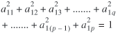
As described in Washington et al. (2003), EFA is not a statistical model and there is no distinction between dependent and independent variables in this analysis. For the EFA is to be useful, there are K < n factors or principal components, with the first factor given as
Z 1 = a 1 1 x 1 + a 1 2 x 2 + … + a 1 q x q
+ … + a 1 (p - 1) y (p - 1) + a 1 p y p (1)
which maximizes the variability across individuals, subject to the constraint
 (2) (2)
where observed variables are denoted by (p × 1) column vector y, and (q × 1) column vector x, and influence the latent endogenous and exogenous variables, respectively. Thus, VAR[Z1] is maximized given the constraints in equation (2), with the constraints imposed to ensure determinacy. A second factor, Z2, is then sought to maximize the variability across individuals, subject to the constraints
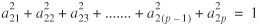
and COR[Z1,Z2] = 0, and so on, such that COR[Z1, Z2.......ZK] = 0 for up to K factors. In this paper, the various survey responses are the observed variables, and they are used to identify the underlying latent variables. Manly (1986), Johnson and Wichern (2002), and Washington et al. (2003) provide additional details of EFA.
After identifying useful factors from EFA, SEMs are developed. A SEM is defined with two components, a measurement model and a structural model. SEMs are a natural extension of factor analysis and are used to identify structural relationships between latent as well as observed variables. The measurement model portion of a SEM correlates the observed variables with latent dependent, as well as independent, variables. Observed variables influencing latent endogenous and exogenous variables are denoted by a (p × 1) column vector of y and (q × 1) column vector of x, such that
y = Λ y η + ε (3)
x = Λ x ξ + σ (4)
where
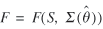
Λy(p × m) and Λx(q × n) are the coefficient matrices that show the relation of y to η and x to ξ, respectively, and ε(p × 1), and δ(q × 1) are the errors of measurement for y and x, respectively (Washington et al. 2003). For example, if statewide safety is a latent dependent variable of interest, it is denoted as η and all the observed variables, such as alcohol-related fatalities, pedestrian and bicycle-related fatalities, etc., would constitute the y vector.
The structural component of a SEM is given as
η = Β η + Γ ξ + ς (5)
where
η is an (m × 1) vector of latent endogenous random variables,
ξ is a vector of (n × 1) latent exogenous random variables,
B is an (m × m) coefficient matrix reflecting the influence of the latent endogenous variables on each other,
Γ is an (m × n) coefficient matrix for the effects of ξ on η, and
ς is the vector of regression errors for which [E(s) = 0] and is uncorrelated with ξ. In addition, the error terms of the measurement models are assumed to be uncorrelated with ξ and ς.
From the previous simultaneous equation (5), and treating all the observed variables as dependent variables in the model, the covariance matrix is given as
Σ (θ) = G (I - β) -1 γ φ γ (I - β) (-1)′ G′ (6)
where G is the selection matrix containing either zero or one to select the observed variables from all the dependent variables in η. Once the SEM model is identified (statistically), the parameters are estimated using a discrepancy function based on the hypothesized model Σ = Σ(θ), where Σ is estimated by the sample covariance matrix S. The role of this discrepancy function is to minimize the difference between the sample variance-covariance matrix and the model-implied variance-covariance matrix, and is given as
 (7) (7)
It is important to note that the observed variables in this study are mainly categorical in nature and are not approximated well by normal distributions. According to Bollen (1989), the weighted least squares (WLS) estimator has the desirable property of making minimal assumptions about the distribution of observed variables, unlike maximum likelihood estimators (MLEs), which presuppose the underlying data to be approximately normally distributed. Hence, we used the WLS estimator instead of MLE for this research. The fitting function for WLS is
F WLS = [s - (θ)]′ W -1 [s - σ (θ)] (8)
where
s is a 1/2(p + q)(p + q + 1) vector containing the polychoric and polyserial correlation coefficients for all pairs of latent endogenous and observed exogenous variables,
σ(θ) is the corresponding same-dimension vector for the implicated covariance matrix, and
W is a consistent estimator of the asymptotic covariance matrix of s.
Goodness-of-Fit Measures
To evaluate the overall goodness of fit of the estimated models, χ2 fit, the root mean square error of approximation (RMSEA), normed fit index (NFI), and Tucker-Lewis index (TLI) were calculated and used to guide final model selection. In this context, it is important to mention that goodness of fit in SEM is an unsettled topic for which many researchers have presented a variety of viewpoints and recommendations. While a detailed explanation of them is beyond the scope of this paper, a brief description about each measure of fit used in this paper is provided.
As described by Washington et al. (2003), a useful feature of discrepancy functions is that they can be used to test the null hypothesis H0 :Σ(θ) = Σ, and (n – 1) times the discrepancy function evaluated at  is approximately χ2 distributed. The degrees of freedom are 1/2(p + q)(p + q + 1) – t, where p and q are as described previously, and t is the number of free parameters in θ. This χ2 divided by model degrees of freedom has been suggested as a useful goodness-of-fit measure. However, in this context, the logic of significance testing is different from significance of coefficient testing in a regression equation (Bollen 1989). In the classical application, we hope to reject the null hypothesis, whereas in the SEM (for the χ2 test) the null hypothesis assumes that the implied model is equal to the true model and we do not wish to reject it. As a result, a large χ2 and small p value suggests model lack of fit. Thus, a relatively large p value and small χ2 is sought and corresponds to a good fit of the model-implied variance-covariance with the observed one. is approximately χ2 distributed. The degrees of freedom are 1/2(p + q)(p + q + 1) – t, where p and q are as described previously, and t is the number of free parameters in θ. This χ2 divided by model degrees of freedom has been suggested as a useful goodness-of-fit measure. However, in this context, the logic of significance testing is different from significance of coefficient testing in a regression equation (Bollen 1989). In the classical application, we hope to reject the null hypothesis, whereas in the SEM (for the χ2 test) the null hypothesis assumes that the implied model is equal to the true model and we do not wish to reject it. As a result, a large χ2 and small p value suggests model lack of fit. Thus, a relatively large p value and small χ2 is sought and corresponds to a good fit of the model-implied variance-covariance with the observed one.
Another class of goodness-of-fit measures available in SEM is based on the population discrepancy function as opposed to the sample discrepancy function, such as RMSEA. The RMSEA is obtained by taking the square root of the population-based discrepancy function divided by its degrees of freedom. Practical experience indicates that a value of RMSEA of about 0.05 or less indicates a good fit of the model.
The remaining two goodness-of-fit measures are based on comparisons with a baseline model. The NFI proposed by Bentler and Bonett (1980) indicates the level of improvement in the overall fit of the present model compared with the baseline model and is given as
 (9) (9)
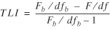
where F and Fb are the discrepancy functions of the fitted and baseline models. The TLI is similar to this concept, but in addition to the discrepancy functions, the degrees of freedom associated with the fitted model (df), as well as the baseline model (dfb), are considered in calculating the index, thus a penalty can be imposed for larger models similar to an adjusted R2 in regression. The index is given as
More information on SEM estimation, goodness of fit, variable selection, specification, and interpretation can be found in Bollen (1989), Arminger et al. (1995), Hoyle (1995), Schumacker and Lomax (1995), Kline (1998), and Washington et al. (2003).
SEM MODEL STARTER SPECIFICATION
The hypotheses mentioned previously, and described in greater detail here, helped to provide the research team with an initial SEM specification.
Hypothesis 1. The breadth and depth of statewide programs should in theory influence statewide safety, albeit with a time lag. It is hypothesized that states with relatively poor safety records will have broad and intensive safety programs, in response to a needed safety improvement. This finding would reflect an appropriate allocation of federal funds for improving safety across states. Because changes in statewide safety typically are not immediate, and because program benefits tend to lag program investments, it is assumed that depth and breadth of safety programming will be negatively associated with statewide safety. This anticipated relationship is aggregate in nature and exceptions may occur.
Hypothesis 2. GHSAs that perceive benefits from participating in the transportation planning process will be more likely to adopt a coordinated approach to safety and will, consequently, be more likely to identify new opportunities for addressing safety, thereby yielding increased safety performance. Understanding how these agencies develop their perceptions of planning activities is difficult to assess. For instance, an unfavorable attitude could represent an institutional unwillingness to coordinate with other agencies or may be the result of a previously unsuccessful attempt at coordinating with other agencies. Alternatively, a positive perception of planning may be the result of successful experiences in previous coordination attempts or may simply represent an appreciation for the potential benefits of a coordinated approach. It could also represent a latent agency willingness to adopt new and innovative approaches to transportation safety, even if the agency has never previously attempted to coordinate their efforts with planning entities. It is hypothesized that in aggregate, agencies with a positive perception of planning are expected to be willing to introduce a broad range of programs addressing safety, as well as yield better than average safety records.
Although these hypotheses represent a priori beliefs about the relationships between latent variables and guided the specification of the structural relationships in the SEM models, the latent factors were identified through an EFA. The survey response—observed endogenous variables (endogenous because they are influenced by the underlying latent variables)—form the x and y vectors in equation (1) and may be related to one or more latent variables. The factor loadings give an indication of how many distinctly different "dimensions" exist in the data.
The exploratory factor analysis output (table 2) clearly shows significant loadings for some variables on a specific factor compared with others. For example, the variable PEDS2 loads significantly on the first factor but not on the second and third factors. These differences in factor loadings help the analyst to determine which observed variables are influenced by a common underlying factor, how many latent variables to consider in a SEM, and how to specify the measurement portion of a SEM (e.g., which observed endogenous variables measure the latent variables). The EFA in this study produced strong evidence in support of three latent variables, which are described as:
- Breadth of the programs (PROGRAM in figure 1). This latent variable reflects the extent of programs reported by GHSAs around the United States. The questions that loaded heavily (were influenced by breadth of programs) on this factor included Q2a–Q2e, Q9a–Q9c, and Q10a–Q10d, survey responses that describe agency goals for pedestrian and bike safety programs, education, and enforcement.
- Attitude of the agencies toward planning (ATTITUDE_PLN in figure 1). This latent variable influences collectively the responses to questions Q13a–Q13g, Q14a, Q15a, and Q16a, which represent attitudinal and perception-related questions.
- Risk. This latent variable is strongly associated with variables such as total and alcohol-related crash rates and pedestrian and bicycle-related crash rates. Thus, the variable reflects the amount of motor vehicle-related risk across the states. It is worthwhile to note that the observed crash rates measure the degree that something is not safe, and thus the latent variable is labeled RISK.
RESULTS
Using Mplus software, we obtained the results of the SEM estimated on the survey and statewide crash data. The relationships among the observed and latent variables are shown in figure 1. For ease of understanding, the observed endogenous variables are shown as rectangles, while both latent endogenous and exogenous variables appear as ellipses. The circles represent the unobserved measurement error terms. Arrows in the diagram suggest the direction of influence, thereby identifying the endogenous and exogenous variables. For example, the base of an arrow is attached to an exogenous variable while the variable to which it points is endogenous. A similar concept is also valid for the error terms. A 0 next to a variable indicates that its mean is set to 0 and the 1 near the arrow means the regression weight is given as 1. There must also be at least two observed endogenous variables pointing to a latent variable for identifiability of the model (a necessary condition for ensuring that sufficient information exists to estimate the model parameters).
Overall Model Goodness-of-Fit
As discussed previously, the hypothesized relationships between variables were used to identify structural relationships, while survey questions and state-level crash data were used to formulate the measurement portion of the model. The latent variables in the starter specification model were loaded with all the significant variables obtained from the exploratory factor analysis based on the factor loadings. A variable with a factor loading of greater than 0.5 was considered significant and included in the model. However, including all of the significant observed variables in the measurement model resulted in non-identifiability of the model (too many model parameters relative to the data to estimate).
As a result, an iterative process was adopted where the "least" significant variables were removed and an improved SEM model was obtained based on the model fit and convergence criteria. Note that changes during this process were made only to the measurement model and not to the structural model relating latent variables. For example, TOLFTVMT, which presents the total number of crashes per VMT, was dropped from the final model, because a better fitting model was achieved using three other accident-related variables explaining the latent variable RISK. Deleting TOLFTVMT from RISK was not detrimental to model fit, as it explains the total crash including pedestrian, bike, and alcohol-related accidents, and these were already taken into consideration by the other three observed variables. The problem of restricting the measurement models to a few select variables was dependent on sample size and model complexity and is addressed in the section on further research.
Table 3 shows the final SEM specification results. The interpretation of the results in the table is straightforward and consistent with the arrows-between-variables explanation of figure 1. The first row in table 3 shows that the latent variable PROGRAM acts as an exogenous variable on the latent variable RISK with a coefficient estimate of 0.026, standard error of 0.021, and t value of 1.226. The second part of table 3 presents the estimated intercepts of the observed endogenous variables.
Table 4 shows various goodness-of-fit statistics used during model selection. The chi-square value for the final model is 15.455 with 17 degrees of freedom (p value of 0.5627), which indicates the model fit cannot be rejected at p
= 0.05. Because the chi-square goodness-of-fit test is used to test for differences between the implied model variance-covariance matrix and the observed one, a model that will not reject the null hypothesis is a desired outcome. The RMSEA for the final model was 0.003, which clearly indicates a close-fitting model. Also, the calculated NFI and TLI are close to 1, indicating considerable improvement over the baseline model.
General Findings
The model results suggest a two-way relationship between risk and the program efforts by GHSAs, or that these two aspects are mutually endogenous. Risk affects programming, and programming also affects risk. States with high safety risk actively implemented a wide variety of safety programs resulting in a breadth of the programs being positively associated with safety risk. This finding agreed with expectations that relatively higher safety risk drives the allocation of federal funding and thereby supports a broad range of safety programs targeted toward safety improvements. Also, the effect of risk on programming is significantly larger than the effect of programming on risk. This suggests there is a considerable lag between safety investments and risk reductions, or the combinations of safety programs do not bring about risk reductions proportionate to the effect of risk on programming. The squared multiple correlations (R2 statistics) for the latent variables RISK and PROGRAM are 0.686 and 0.431, respectively, indicating that the model explains 68% of the variance in PROGRAM and 43% of the variance in RISK.
The latent variable ATTITUDE_PLN, which captures GHSAs' attitudes toward integrating state safety programs with transportation-related activities, as well as their participation in regional transportation planning, was positively associated with PROGRAM
. The model also suggests that the attitude of GHSAs directly affects the latent variable PROGRAM and indirectly affects the exogenous variable RISK through PROGRAM
. These findings imply that a positive attitude toward safety planning within GHSAs results in a broader and more extensive implementation of safety programs by GHSAs. This result again confirmed a priori expectations that agencies active in safety planning would be likely to implement a broad range of programs to improve statewide transportation safety.
CONCLUSIONS
ISTEA and the TEA-21 legislation raised the visibility of safety conscious planning in the United States. While safety-related planning has historically been reactive, new initiatives and investments are intended to change the status quo and encourage a new approach for considering safety at the transportation planning level. In particular, the NCHRP 8-44 project is oriented toward contributing and understanding tools for proactive planning among DOTs, MPOs, and GHSAs. This paper presents an exploratory analysis aimed at better understanding the relationships between GHSA-implemented safety programs and the actual safety scenario, as well as the effect of coordination among the various agencies on statewide safety.
The study revealed that coordination of transportation safety across DOTs, MPOs, GHSAs, and departments of public safety appears to be generally beneficial to safety, particularly in the long term. In addition, better safety planning coordination is characterized by positive attitudes toward incorporating safety into planning and also implementing a wide range of programs to improve safety. Furthermore, mechanisms for improving cooperation, coordination, and collaboration among the agencies also appear to be worthwhile investments.
FUTURE WORK
The results presented in this paper are exploratory due to a lack of a well-articulated theory regarding the subject matter. Additional information and some controlled data-collection would be required to draw more definitive conclusions. For example, panel data over a period of 5 to 10 years would be required to examine the lag between safety investments and risk, as well as attitudes and programs implemented over time. Additional data from all 50 states would sufficiently increase the number of observations necessary to improve the WLS estimates obtained in this analysis, allowing for more "complex" models. The WLS estimator requires at least 1/2(p + q)(p + q + 1) observations where (p + q) are the number of observed dependent variables. Hence, the explanatory power of the model greatly depends on the number of observations.
This study was restricted to three main latent variables and a few carefully selected observed endogenous variables in the measurement model, due partly to data limitations. A larger study would enable the research team to focus on perhaps other relevant variables critical to statewide safety performance, such as the types of programs implemented. As a result, the present model remains speculative and further data are needed to validate it. Furthermore, the results are time dependent, due to the observed response from the 2002 to 2003 time periods. As mentioned previously, there is every possibility of a lagged effect of safety improvement programs on state safety performance, which is not properly captured in this modeling effort. Regardless, some initial insights into relationships among agencies were found and are encouraging for the successful implementation of ISTEA and TEA21 legislation targeted towards national safety improvements.
ACKNOWLEDGMENTS
The authors would like to acknowledge the National Cooperative Highway Research Program (NCHRP 8-44) for providing the funding for this research. This paper represents interim preliminary findings that have not been reviewed nor are endorsed by the NCHRP, its staff, or the panel overseeing this research effort.
REFERENCES
Amato, P.R. and B. Alan. 1995. Changes in Gender Role Attitudes and Perceived Marital Quality. American Sociological Review 60(1):58–66.
Arminger, G., C. Clogg, and M. Sobel. 1995. Handbook of Statistical Modeling for the Social and Behavioral Sciences. New York, NY: Plenum Press.
Ben-Akiva, M., F. Humplick, S. Madanat, and R. Ramaswamy. 1991. Latent Performance Approach to Infrastructure Management. Transportation Research Record 1311:188–195.
Bentler, P.M. and D.G. Bonett. 1980. Significance Tests and Goodness of Fit in the Analysis of Covariance Structures. Psychological Bulletin 88:588–606.
Bollen, K.A. 1989. Structural Equations with Latent Variables. New York, NY: Wiley.
Everitt, B.S. 1984. An Introduction to Latent Variables. London, England: Chapman & Hall.
Golob, T.F. and A. Regan. 2000. Freight Industry Attitude Towards Policies to Reduce Congestion. Transportation Research E 36(1):55–77.
Hoyle, R., ed. 1995. Structural Equation Modeling: Concepts, Issues, and Applications. Thousand Oaks, CA: Sage Publications, Inc.
Insurance Institute for Highway Safety (IIHS). 2004. Available at http://www.hwysafety.org/safety_facts/safety.htm.
Johnson, R. and D. Wichern. 2002. Applied Multivariate Statistical Analysis. Upper Saddle River, NJ: Prentice Hall.
Kline, R. 1998. Principles and Practice of Structural Equation Modeling. New York, NY: Guilford Press.
Loehlin, J.C. 2004. Latent Variable Models: An Introduction to Factor, Path, and Structural Equation Analysis. Mahwah, NJ: Lawrence Erlbaum Associates.
Manly, B. 1986. Multivariate Statistical Methods: A Primer. New York, NY: Chapman & Hall.
Molenaar, K., S. Washington, and J. Dickmann. 2000. Structural Equation Model of Construction Contract Dispute Potential. Journal of Construction Engineering and Management, July/August:1–10.
Östberg, M. and B. Hagekull. 2000. A Structural Modeling Approach to the Understanding of Parenting Stress. Journal of Clinical Child Psychology 29(4):615–625.
Rubio, D.M., M.B. Weger, and S.S. Tebb. 2001. Using Structural Equation Modeling to Test for Multidimensionality. Structural Equation Modeling: A Multidisciplinary Journal 8(4):613–626.
Schumacker, R.E. and R.G. Lomax. 1995. A Beginner's Guide to Structural Equation Modeling. Mahway, NJ: Lawrence Erlbaum Associates.
U.S. Department of Transportation (USDOT), National Highway Traffic Safety Administration. 2001. Traffic Safety Facts 2001. Washington, DC.
Washington, S., M. Karlaftis, and F. Mannering. 2003. Statistical and Econometric Methods for Transportation Data Analysis. Boca Raton, FL: Chapman & Hall/CRC.
APPENDIX
Survey Questionnaire
Survey Question 1: Is your agency located within, or directly affiliated with, another state agency, such as the Department of Transportation?
1a. affil1—Affiliated with another state agency?
1 = Yes
0 = No
1b. agency1—Name of affiliated agency.
1c. agcycod—Coding of agency affiliation.
0 = No affiliation
1 = State DOT
2 = State police
3 = Department of Public Safety
4 = Department of Motor Vehicles
5 = Other affiliation
Survey Question 2: Do your agency's mission statement, goals, or objectives explicitly address any of the following issues?
2a. peds2—Pedestrian safety.
2b. bikes2—Bicycle safety.
2c. drived2—Driver education.
2d. schooled2—Safety education in school.
2e. enforce2—Traffic law enforcement.
2f. coopdot2—Cooperation with the state DOT.
2g. cooploc2—Cooperation with local officials.
2h. coopplan2—Interaction with regional or local transportation planners.
2i. safdes2—Incorporating safety into the design of transportation facilities.
2j. safops2—Incorporating safety into transportation facility operation.
2k. data2—Collecting safety-related data.
1 = Yes
0 = No
Survey Question 3: How many professional staff members (i.e., those focused on highway safety, not clerical or support staff) does your agency have?
Staff3—Number of agency employees.
Survey Question 4: Do any members of your staff have expertise in the following areas?
4a. Eng4—Transportation engineering.
4b. plan4—Transportation planning.
4c. ops4—Traffic operations.
4d. enf4—Law enforcement.
4e. edu4—Education.
4f. mktg4—Marketing/media relations.
1 = Yes
0 = No
Survey Question 5: Federal regulations require Governors Highway Safety agencies to develop annual plans, as well as performance measures for evaluating program effectiveness. How important are these performance measures in influencing the types of projects and programs implemented by your organization?
perfms5—Importance of annual performance measures on agency projects.
5 = Very important
4 = Somewhat important
3 = No opinion
2 = Not very important
1 = Not at all important
Survey Question 6: Are your agency's performance measures shared by other agencies responsible for the transportation system (e.g., by the state DOT or by regional transportation planning agencies in your state)?
6a. Sharepm6—Other agencies sharing performance measures.
1 = Yes
0 = No
6b. agency6—Names of agencies sharing performance measures, if any.
Survey Question 7: Does your agency develop longer term performance targets beyond the federally required 1-year targets?
7a. perftgt7—Performance targets beyond federal requirements.
1 = Yes
0 = No
7b. tgtyear7—Furthest target year in future.
Survey Question 8: What is the planning time horizon for your agency?
Agyhzn8—Agency planning horizon.
Survey Question 9: Which of the following pedestrian-related safety programs does your agency implement?
9a. Pededu9—Education on safe street crossing.
9b. pedcrwk9—Crosswalk enforcement.
9c. pedschl9—Safe routes to schools program.
1 = Yes
0 = No
9d. other9—Other pedestrian programs, if any.
Survey Question 10: Which of the following bicycle-related safety programs does your agency implement?
10a. Bikedu10—Bicycle education campaigns.
10b. bkhelm10—Bicycle helmet programs.
10c. bklite10—Lights on bicycles at night.
10d. bkbrk10—Bicycle brake requirements.
1 = Yes
0 = No
10e. other10—Other bicycle programs, if any.
Survey Question 11: Has your agency undertaken any innovative safety programs using federal flexible funds, such as Section 407 funds that provide flexible incentive grants for programs aimed at increasing highway safety?
11a. Innov11—Innovative programs using flexible funds.
1 = Yes
0 = No
11b. prgrm111—Name of innovative program 1, if any.
11c. effct111—Effectiveness of program.
5 = Very effective
4 = Somewhat effective
3 = No opinion
2 = Somewhat effective
1 = Not effective
11d. prgrm211—Name of innovative program 2, if any.
11e. effct211—Effectiveness of program 2.
5 = Very effective
4 = Somewhat effective
3 = No opinion
2 = Somewhat effective
1 = Not effective
Survey Question 11 (continued): Has your agency undertaken any innovative safety programs using federal flexible funds, such as Section 407 funds that provide flexible incentive grants for programs aimed at increasing highway safety?
11f. prgrm311—Name of innovative program 3, if any
11g. effct311—Effectiveness of program 3.
5 = Very effective
4 = Somewhat effective
3 = No opinion
2 = Somewhat effective
1 = Not effective
11h. prgrm411—Name of innovative program 4, if any.
11i. effct411—Effectiveness of program 4.
5 = Very effective
4 = Somewhat effective
3 = No opinion
2 = Somewhat effective
1 = Not effective
11j. prgrm511—Name of innovative program 5, if any.
11k. effct511—Effectiveness of program 5.
5 = Very effective
4 = Somewhat effective
3 = No opinion
2 = Somewhat effective
1 = Not effective
Survey Question 12: This study seeks to understand how often your agency interacts with other individuals, agencies, or groups that may have an influence on highway safety issues. For each of the following, please indicate whether your agency interacts with them monthly, once every three months, once every six months, once per year, or not at all.
12a. Dot12—Frequency of interaction with the state DOT.
12b. spolce12—Frequency of interaction with the state police.
12c. lpolce12—Frequency of interaction with the local police.
12d. plan12—Frequency of interaction with MPOs.
12e. legs12—Frequency of interaction with state legislators.
12f. gov12—Frequency of interaction with the governor's staff.
12g. hwy12—Frequency of interaction with highway contractors.
12h. engnr12—Frequency of interaction with engineering consultants.
12i. school12—Frequency of interaction with school officials.
12j. local12—Frequency of interaction with local officials.
4 = At least monthly
3 = Once every three months
2 = Once every six months
1 = Once per year
0 = Never
Survey Question 13: Has your agency considered integrating state safety programs with any of the following transportation-related activities:
13a. Sdwlk13—Considered sidewalk provisions.
13b. crswlk13—Considered crosswalk signals.
13c. bike13—Considered bike signals.
13d. speed13—Considered design strategies to reduce speeding.
13e. turn13—Considered design strategies to prevent turning movements.
13f. rdside13—Considered eliminating roadside hazards.
13g. monitr13—Considered using monitoring systems.
1 = Yes
0 = No
Survey Question 14: Every urbanized area in a state must have a comprehensive regional transportation planning process. For such areas in your state, has your agency participated in the regional transportation planning process during the last 5 years?
14a. mpo14—Participated in regional transportation planning during the last 5 years.
1 = Yes
0 = No
If mpo14 = 0
14b. blrp14—Benefited from participating in MPO long-range planning process (if no 14mpo).
1 = Yes
0 = No
14c. bgopm14—Benefited from developing MPO goals, objectives, and performance measures (if no 14mpo).
1 = Yes
0 = No
14d. bpep14—Benefited from participating in MPO project evaluation and programming (if no 14mpo).
1 = Yes
0 = No
Survey Question 15: Many states have regional planning agencies that represent rural,
non-urbanized portions of a state. Has your agency participated in the transportation planning process for rural areas during the last 5 years?
15a. Rural15—Participated in rural planning process during the last 5 years.
1 = Yes
0 = No
If rural15 = 0
15b. blrp15—Benefited from participating in rural long-range planning process (if no 15rural).
15c. bgopm15—Benefited from developing rural goals, objectives, and performance measures (if no 15rural).
15d. bpep15—Benefited from participating in rural project evaluation and programming (if no 15rural).
1 = Yes
0 = No
Survey Question 16: Every state has a statewide transportation planning process that, at a minimum, is responsible for producing a state transportation plan. Has your agency participated in the statewide transportation planning process during the last 5 years?
16a. 16stp—Participated in state transportation planning process during the last 5 years.
1 = Yes
0 = No
If stp16 = 0
16b. blrp16—Benefited from participating in state long-range planning process (if no 16stp).
16c. bgopm16—Benefited from developing state goals, objectives and performance measures (if no 16stp).
16d. bpep16—Benefited from participating in state project evaluation and programming (if no 16stp).
1 = Yes
0 = No
Survey Question 17: To what extent does the transportation planning process in your state influence the programs or initiatives undertaken by your agency?
Influ17—Influence of transportation planning process on highway safety programs.
2 = Strongly influences
1 = Moderately influences
0 = Does not influence
9 = Don't know
ADDRESSES FOR CORRESPONDENCE
1 Corresponding author: S. Mitra, Department of Civil and Environmental Engineering, Arizona State University, PO Box 875306, Tempe, AZ 85287-5306. E-mail: mitra_sudeshna@yahoo.com
2 S. Washington, Department of Civil and Environmental Engineering, Arizona State University, PO Box 875306, Tempe, AZ 85287-5306. E-mail: Simon.Washington@asu.edu
3 E. Dumbaugh, School of Civil and Environmental Engineering, Georgia Institute of Technology, Atlanta, GA 30332-0355. E-mail: EDumbaugh@aol.com
4 M. Meyer, School of Civil and Environmental Engineering, Georgia Institute of Technology, Atlanta, GA 30332-0355. E-mail: mmeyer@ce.gatech.edu
|