Robust Estimation of Origin-Destination Matrices
Byron J. Gajewski*
The University of Kansas
Laurence R. Rilett
Texas A&M University and Texas Transportation Institute
Michael P. Dixon
University of Idaho
Clifford H. Spiegelman
Texas A&M University and Texas Transportation Institute
ABSTRACT
The demand for travel on a network is usually represented by an origin-destination (OD) trip table or matrix. OD trip tables are typically estimated with synthetic techniques that use observed data from the traffic system, such as link volume counts from intelligent transportation systems (ITS), as input. A potential problem with current estimation techniques is that many ITS volume counters have a relatively high error rate. The focus of this paper is on the development of estimators explicitly designed to be robust to outliers typically encountered in ITS. Equally important, standard errors are developed so that the parameter reliability can be quantified.
This paper first presents a constrained robust method for estimating OD split proportions, which are used to identify the trip table, for a network. The proposed approach is based on a recently developed statistical procedure known in the literature as the L2 error (L2E). Subsequently, a closed-form solution for calculating the asymptotic variance associated with the multivariate estimator is derived. Because the solution is closed form, the computation time is significantly reduced as compared with computer-intensive standard error calculation methods (e.g., bootstrap methods), and therefore confidence intervals for the estimators in real time can be calculated. As a further extension, the OD estimation model incorporates confirmatory factor analysis for imputing origin volume data when these data are systematically missing for particular ramps. The approach is demonstrated on a corridor in Houston, Texas, that has been instrumented with ITS automatic vehicle identification
readers.
INTRODUCTION
The demand for travel on a network is usually represented by an origin-destination (OD)
trip table or matrix. A trip is a movement from one point to another, and each cell, ODkj, in the table represents the number of trips starting at origin k and ending at destination j. An OD trip table is a required input to most traffic operational models of transportation systems. In addition, demand estimates are useful for real-time operation and management of the system. While it would be possible to directly measure the travel volume between two points, it is a very expensive and time-consuming process to identify the
trip matrix for an entire network. Consequently, OD trip volume tables are typically estimated with synthetic techniques that use observed data from the traffic system, such as link volume counts from inductance loops, as input. Over the past 20 years, numerous methodologies have been proposed for estimating OD movements within an urban environment (Bell 1991;
McNeil and Henderickson 1985; Cascetta 1984). A common approach for estimating OD volumes is based on least squares (LS) regression where the unknown parameters are estimated based on the minimization of the Euclidean squared distance between the observed link volumes and the estimated link volumes. Deriving OD trip tables from intelligent transportation systems (ITS) volume data is the focus of this paper.
Nihan and Hamed (1992) demonstrated that outlier data can have a significant impact on OD estimate accuracy, but most OD estimation techniques assume that the input data are reliable. Furthermore, it has been shown that unless inductance loops are maintained and calibrated at regular intervals, the data received from them are prone to error rates of up to 41% (Turner et al. 1999). Faulty volume counts can occur because of failures in traffic monitoring equipment, communication failure between the field and traffic management, and failure in the traffic management archiving system. The first two failure types may be difficult to detect because they occur in isolated detectors. Other detector problems include stuck sensors, chattering, pulse breakup, hanging, and intermittent malfunctioning. Consequently, there is a need to account for the input error in the estimation process. Historically, detector malfunctions have been addressed by “cleaning” the datasets prior to the estimation step. This is
problematic for ITS applications, because the data manipulation takes time and the use of these techniques is limited in a real-time environment. Even for off-line applications, cleaning the data is problematic, because it is not always clear which data need to be cleaned and how this can best be accomplished. This paper examines a robust approach whereby the data error associated with the faulty input data is accounted for explicitly within the estimation of the OD trip table.
The development of OD estimators that are robust to detector malfunction has been largely ignored in OD estimation research, with the exception of an approach proposed using a least absolute norm (LAN) estimator (Sherali et al. 1997). LAN is intuitively more robust to outliers than LS, because the errors are not squared as they are in LS (Cascetta 1984; Maher 1983; Robillard 1975), nor are the data treated as constraints as they are in many maximum entropy and information minimization approaches (Cascetta and Nguyen 1988; Van Zuylen 1980). This paper follows on their work by using estimators explicitly designed to be robust to outliers typically encountered in an ITS environment. Equally important, standard errors will be developed so that parameter reliability can be quantified.
This paper first presents a constrained robust method for estimating OD split proportions, which are used to identify the trip table, for a network. The traffic volumes are assumed to come from an Advanced Traffic Management System (ATMS), and the traditional assumption that the data are “reliable” is relaxed to allow the possibility of missing or faulty detector data. The proposed approach is based on a recently developed parametric statistical procedure known in the literature as the L2
error (L2E).1 Subsequently, a closed-form solution for calculating the asymptotic variance associated with the multivariate estimator is derived. Because the solution has a closed form, the computation time is significantly reduced as compared with the computer-intensive calculation of the standard errors (e.g., bootstrap methods and off-line methods based on the LS (Ashok 1996)), and therefore confidence intervals for the estimators in real time can be calculated. As a further
extension, the OD estimation model incorporates confirmatory factor analysis (Park et al. 2002) for imputing volume data when this information is systematically missing for particular ramps.
While the techniques demonstrated here are motivated using inductance loop data, they are easily generalized to other detectors, models, and data. The approach is demonstrated on a corridor in Houston, Texas, that has been instrumented with automatic vehicle identification (AVI) readers. The AVI volumes are used to estimate an AVI OD matrix. The benefit to this test bed is that the actual AVI OD table can be identified and, therefore, provides a unique opportunity for directly measuring the accuracy of the different techniques. The OD matrix can be obtained using a linear combination of the split proportion matrix and the origin (entrance) volume vector.
It should be noted that because the input volumes are dynamic, the estimated OD matrix is also dynamic. However, because the split proportion is assumed constant, the OD matrices by time slice are linear functions of each other.
Also note that while the method is acceptable for freeway networks with relatively short trips between interchanges, such as the example in this paper, an application to a larger network would raise the question as to when the trips began or ended. Caution should be exercised when applying this method to a large proportion of trips that begin and end during different time periods.
THEORY
The objective of this paper is to estimate the OD split proportion matrix and its associated distribution properties. The split proportion Pkj is defined as the proportion of vehicles that exit the system at destination ramp j given that they enter at origin ramp k. While the split proportions are estimated using only the volumes observed at the origins and destinations, the approach can easily be extended to the case where general lane volumes are observed as well. Once the OD split proportion matrix is identified, the OD table can be derived. See the appendix for a notation list and all proofs of the theorems.
Methodology
A desirable feature of an OD estimator is the ability to calculate a closed-form limiting distribution. This is particularly important for ITS applications, so that confidence intervals about the estimate can be calculated in real time. The estimator will be defined and distributional properties of the estimator will be derived following the steps below.
- Define the multivariate constrained regression model and objective functions.
- Obtain distributional properties.
- Stack the variables to obtain a univariate constrained regression model.
- Use the equality constraints to obtain a univariate unconstrained regression model.
- Apply asymptotic theory to derive the distributions of the estimated split proportions for the LS and the L2E estimation
techniques.
- Transform the model back to its original form.
Step 1: Define the Model and
Objective Functions
A traffic network can be represented by a directed graph consisting of arcs (or links)
representing roadways and vertices (or nodes) representing intersections. There are q
origin (entrance) ramps and p destination (exit) ramps, and the analysis period is broken
down into T time periods of equal
length  t.
Figure 1 shows an example of a traffic system in
Houston, Texas, along the inbound (eastbound) Interstate 10 (Katy Freeway) corridor and a schematic diagram of the corridor. t.
Figure 1 shows an example of a traffic system in
Houston, Texas, along the inbound (eastbound) Interstate 10 (Katy Freeway) corridor and a schematic diagram of the corridor.
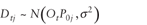
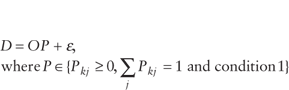
The underlying assumption of the OD model developed here is that mass conservation holds. In essence, it is assumed that the traffic entering the system also exits the system within a specified time period. This assumption is appropriate as long as the time intervals are long and/or the traffic is in a steady state. For time period t, t = 1, 2,…,T, Dtj denotes the destination volume at destination ramp j, j = 1,2,3,…,p and Otk denotes the origin volume at origin ramp k, k = 1,2,3,…,q.
The first assumption is that the split proportion Pkj is constant over the entire analysis period. The second assumption is that the number of vehicles entering the system equals the number of vehicles exiting the system so that the split proportions at each origin during the period sum
to 1 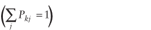 . The expectation of the destination volumes during each time
period t is a linear combination of the split proportions weighted by the origin volumes . The expectation of the destination volumes during each time
period t is a linear combination of the split proportions weighted by the origin volumes

The term  is the error. is the error.
Intuitively, some of the split proportions are not feasible (Pkj = 0) because of the structure of the traffic network, and this needs to be incorporated in the estimation process. Note that in some cases the nonfeasible parameters may simply represent unlikely cases. The zeros are exact in the applications presented later.
It is assumed in this paper that the errors in each column are independently and identically distributed with mean zero and constant variance. This means that the error associated with the volume measurement at destination j is uncorrelated with the volume measurement at destination j´. Note that all assumptions will be checked in the applications section of the paper.
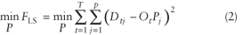
Because the OD problem structure is implicit rather than explicit, and because it is also overspecified, the synthetic approaches attempt to estimate the split proportion matrix based on the minimization of an objective function (Dixon 2000). The objective function in equation 2 is based on an LS approach, which is a common way to estimate the split proportions (Robillard 1975).
Note that if  is distributed normally then the LS is equivalent to the maximum likelihood estimator.
The central hypothesis of this paper is that the LS method is inappropriate for ITS applications because of the high error rate of the measured volumes. In contrast, the L2E objective function is defined as the integrated squared difference between the true probability density function and the estimated density function. Therefore, it is theoretically more robust, relative to the LS, when the data have outliers such as those caused by detector malfunctions. A more specific discussion of this follows.
As an example, consider a sample of size T. If the goal is to estimate the location
parameter, or the central tendency, OtP0 (suppose P0 is
the true unknown split proportion, estimated with P), then the minimization of the integrated
squared error is shown in equation 3 and derived in the appendix,
![minimum over uppercase p (uppercase f subscript {uppercase l subscript {2} uppercase e}) equals minimum over uppercase p [summation from negative infinity to positive infinity [lowercase f (uppercase d subscript {lowercase t j} vertical bar (uppercase o subscript {lowercase t} times uppercase p subscript {lowercase j}))] superscript {2} times lowercase d times uppercase d subscript {lowercase t j} minus [2 divided by (uppercase t times lowercase p) (summation from lowercase t equals 1 to uppercase t summation from lowercase j equals 1 to lowercase p) lowercase f (uppercase d subscript {lowercase t j} vertical bar (uppercase o subscript {lowercase t} times uppercase p subscript {lowercase j}))]]](https://webarchive.library.unt.edu/eot2008/20081022194522im_/http://www.bts.gov/publications/journal_of_transportation_and_statistics/volume_05_number_23/images/gajequNEW3.gif)
The normal distribution,
 ,
replaces ,
replaces  resulting
in the objective function displayed as equation 4, resulting
in the objective function displayed as equation 4,
![minimum over uppercase p (uppercase f subscript {uppercase l subscript {2} uppercase e}) equals minimum over uppercase p [(1 divided by (2 times the square root {lowercase pi} times lowercase sigma)) minus [2 divided by (uppercase t times lowercase p) (summation from lowercase t equals 1 to uppercase t summation from lowercase j equals 1 to lowercase p) (uppercase n (uppercase d subscript {lowercase t j} minus (uppercase o subscript {lowercase t} times uppercase p subscript {lowercase j}, lowercase sigma superscript {2}]]](https://webarchive.library.unt.edu/eot2008/20081022194522im_/http://www.bts.gov/publications/journal_of_transportation_and_statistics/volume_05_number_23/images/gajequ4.gif)
The L2E minimizes the sum of probability density functions (pdfs) while the MLE (or LS) minimizes the negative product of pdfs. In the presence of an outlier, the MLE objective function will multiply a zero and the L2E objective function would add a zero. The relative effect of the outlier on the objective function is much more severe in the case of the MLE. This is because of the multiplicative effect of the zeros on the MLE objective function. Because ITS data often contain outliers, it is hypothesized that the L2E objective function will provide better estimates. For a more detailed discussion of the L2E properties, see Basu et al. (1998) or Gajewski (2000).
When calculating the L2E, an estimate of the variance is required. In this paper, the
estimate of the variance is identified using a two-step process.
First  is calculated using the median of the squared residuals so that an initial estimate of the standard
deviation,
is calculated using the median of the squared residuals so that an initial estimate of the standard
deviation,  ,
may be obtained by calculating the median absolute deviation (MAD) from the set of estimated
residuals, where the tth estimated residual
is ,
may be obtained by calculating the median absolute deviation (MAD) from the set of estimated
residuals, where the tth estimated residual
is 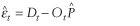 .
The median of the squared residuals is used because it has been shown to have a high breakdown point (Hampel et al. 1986). In general, the breakdown point is the percentage of outliers in the data at which the estimator is no longer robust (Huber 1981). For example, if the breakdown point is 50% then the estimator is robust to datasets that contain less than 50% outliers. .
The median of the squared residuals is used because it has been shown to have a high breakdown point (Hampel et al. 1986). In general, the breakdown point is the percentage of outliers in the data at which the estimator is no longer robust (Huber 1981). For example, if the breakdown point is 50% then the estimator is robust to datasets that contain less than 50% outliers.
Steps 2a–b: Stack and Define
the Unconstrained Univariate Regression Model
Through reparameterization, the split proportion model shown in equation 1 can be translated into an unconstrained univariate regression model. The first step is to stack the split proportion matrix P, where
Pv = vec(P).
For example,
![[2 by 2 matrix where (row 1 column 1 is 1) (row 1 column 2 is 2) (row 2 column 1 is 3) and (row 2 column 2 is 4)] superscript {lowercase v} equals [1 by 4 matrix where (row 1 column 1 is 1) (row 2 column 1 is 3) (row 3 column 1 is 2) and (row 4 column 1 is 4)]](https://webarchive.library.unt.edu/eot2008/20081022194522im_/http://www.bts.gov/publications/journal_of_transportation_and_statistics/volume_05_number_23/images/gajequ4d.gif)
The equality constraints are subsequently defined relative to Pv using GPv = g, where the
matrices
![uppercase g equals [2 by 1 matrix where (row 1 column 1 is 1 superscript {'} subscript {lowercase p} cross uppercase i subscript {lowercase q}) and (row 2 column 1 is uppercase m)]](https://webarchive.library.unt.edu/eot2008/20081022194522im_/http://www.bts.gov/publications/journal_of_transportation_and_statistics/volume_05_number_23/images/gajapp9.gif) and and
![lowercase g equals [2 by 1 matrix where (row 1 column 1 is 1 subscript {lowercase q}) and (row 2 column 1 is 0 subscript {lowercase r})]](https://webarchive.library.unt.edu/eot2008/20081022194522im_/http://www.bts.gov/publications/journal_of_transportation_and_statistics/volume_05_number_23/images/gajapp14.gif)
The matrix M (r by qp) maps the nonfeasible values of Pv to zero. The value r is the number of split proportions equal to zero.
As an example, define 
where P11 = 0 and P21 = 0.
Therefore, the product of the M and Pv matrix maps the nonfeasible elements to zero

where
![uppercase g p superscript {lowercase v} equals [1 by 2 matrix where (row 1 column 1 is uppercase g subscript {1}) and (row 1 column 2 is is uppercase g subscript {2}] times [2 by 1 matrix where (row 1 column 1 is uppercase p superscript {lowercase v} subscript {1}) and (row 2 column 1 is uppercase p superscript {lowercase v} subscript {2}]](https://webarchive.library.unt.edu/eot2008/20081022194522im_/http://www.bts.gov/publications/journal_of_transportation_and_statistics/volume_05_number_23/images/gajequ5.gif)
The first q rows of each G and g are used to normalize the split proportions as shown in equation 5.
Given the constraints defined above and the stacked model, the reduced model may be obtained by solving equation 5. Because G1 is trivially full rank (q + r):
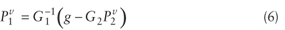
Equation 1 is placed in univariate form by defining Y to be the stacked columns of D and at the same time
letting 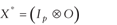 When equation 6 is substituted into the stacked model the unconstrained model is obtained. The substitution is done with the portion of the stacked model that corresponds
to the
When equation 6 is substituted into the stacked model the unconstrained model is obtained. The substitution is done with the portion of the stacked model that corresponds
to the ![uppercase x superscript {star} equals [uppercase x superscript {star} subscript {1} times uppercase x superscript {star} subscript {2}]](https://webarchive.library.unt.edu/eot2008/20081022194522im_/http://www.bts.gov/publications/journal_of_transportation_and_statistics/volume_05_number_23/images/gajapp13.gif) regression parameters. If
regression parameters. If
then 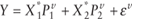
and the new regression model, which describes in univariate form the multivariate regression problem, is defined in equation 7.

where
![uppercase y subscript {2} equals (uppercase y minus (uppercase x superscript {star} subscript {1} times uppercase g superscript {-1} subscript {1} times lowercase g); uppercase w subscript {2} equals [uppercase x superscript {star} subscript {2} minus (uppercase x superscript {star} subscript {1} times uppercase g superscript {-1} subscript {1} times uppercase g subscript {2}].](https://webarchive.library.unt.edu/eot2008/20081022194522im_/http://www.bts.gov/publications/journal_of_transportation_and_statistics/volume_05_number_23/images/gajequ7a.gif)
Step 2c–d: Variance Estimates for
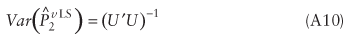
the Reparameterized Model and Distributions
These next steps produce distributions for the estimators under the reparameterized model, in particular that both L2E and LS produce estimators that consistently estimate the
true Pv
(or 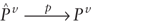 ),
and that ),
and that  is asymptotically normally distributed, under certain assumptions. The asymptotic normality directly produces variance estimates
of .
is asymptotically normally distributed, under certain assumptions. The asymptotic normality directly produces variance estimates
of .
The asymptotic properties follow directly from the reparameterized model discussed in Steps 2a–b. Then the asymptotic theorems from Huber (1981) from the objective functions (or derivatives of them called M-estimators) are applied, written in an unconstrained form.
The only additional assumptions for these asymptotic results are that the errors in equation 1 have a
mean of zero and a variance
of  and are iid. This assumption encompasses many distributions that include heavier tails then the normal distribution. The specific calculations for the asymptotic variances
are
and are iid. This assumption encompasses many distributions that include heavier tails then the normal distribution. The specific calculations for the asymptotic variances
are 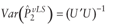 and, and,
![var (uppercase p hat superscript {lowercase v uppercase l subscript {2} uppercase e} subscript {2}) equals (uppercase e [lowercase psi superscript {2}]) divided by ((uppercase e [lowercase psi superscript {'}]) superscript {2}) times (uppercase u superscript {'} times uppercase u superscript {-1},](https://webarchive.library.unt.edu/eot2008/20081022194522im_/http://www.bts.gov/publications/journal_of_transportation_and_statistics/volume_05_number_23/images/gajappNEWF.gif)
where  and U are defined in the appendix.
One result of this is when the errors are normally distributed the ratio of the variances of the L2E estimator and the LS estimator of any element
of

which says that the variance under the L2E estimator is 1.54 times as high as the LS estimator. Therefore, the L2E estimator is actually less efficient than its LS estimator counterpart. However, by applying a heavy-tailed distribution, the result reverses and the L2E estimator is better than the LS estimator. In the subsequent sections, a simulation demonstrates this result.
Conclusion of Theory
The derivation of the asymptotic distributions has shown that explicit closed-form variance estimates exist and that associated standard errors of the split proportions can be calculated in real time. Notice that these theorems can be extended to other types of M-estimators, in addition to the L2E, as long as the assumptions are met.
Note that if the assumptions to derive the closed-form standard errors are not appropriate, then bootstrap methods will be required. The bootstrap is a computer-intensive procedure that uses resamples of the original data to obtain properties such as standard errors. One can use various algorithms to do this, such as case resampling or model-based resampling (Davison and Hinkley 1997).
APPLICATION
Test Bed
The test bed is an eastbound section of Interstate 10 (I-10) located in Houston, Texas, as shown in figure 1. This section of I-10 is monitored as a part of the Houston Transtar Transportation Management Center (TMC) (operated by the Texas Department of Transportation), the Metropolitan Transit Authority of Harris County (METRO), the City of Houston, and Harris County. There are six automatic vehicle identification readers located in the test bed. As instrumented vehicles pass under an AVI reader, a unique vehicle identification number is recorded and sent to a central computer over phone lines. From this information, the average link travel time is calculated and presented to drivers through various traveler information systems. It may be seen in figure 1 that the I-10 test corridor is made up of five AVI links consisting of six “origins” and six “destinations.” Note that each destination may consist of several destination ramps and each origin may consist of several origin ramps, because the AVI
links are defined by the location of the AVI readers and not the physical geometry of the corridor.
The OD methodology developed in this paper was motivated by the assumption that the TMC has access to volume information obtained from point detectors (i.e., inductance loops). However, the models are tested using data obtained from an AVI system because both AVI volumes and split proportions can be identified. This provides a unique opportunity for comparing the accuracy of the OD estimates that are based on volumes obtained at point sources with observed OD split proportions. In this situation, the split proportions are estimated using only the OD volumes from the AVI data.
Based on a preliminary analysis, 18 days in 1996 were used for the analysis
(October 1, 2, 4, 5, 15–19, 22–26, 30, and November 1, 6, and
8).2
The AVI vehicles detected at the origin and destination ramps during the AM peak period (7 am to 9 am) were aggregated into 4 volume counts of 30-minute duration. Therefore, the number of time periods (T) is equal to 72, the number of destinations (p) is 6, and the number of origins (q) is 6. The
AVI volumes were used as input to the LS and the L2E estimators and the resulting
estimates are presented in table 1.
The assumption that the split proportion matrix was constant, which was used in the derivation of the LS and the L2E estimators, was verified by examining the observed AVI split proportion differences across all days and all time periods of the study. Because these observed split proportion differences were within 0.1 for 95% of the estimates, it was judged that the assumption was reasonable for this test case. The observed mean AVI split proportions for the AM peak are shown in table 1.
The correlation coefficients between the observed mean AVI split proportions and the estimated split proportions by the LS and the L2E estimators are 0.961 and 0.960, respectively. These results indicate that both estimators are successful at estimating the OD split proportions. However, the mean absolute percent error (MAPE) between the mean observed split proportion and the estimated split proportions using the LS and the L2E estimators were 44.5% and 51.3%, respectively. These results indicate each method has an approximate error of 50% with respect to individual OD split proportion estimates.
A further analysis of the absolute percent error (APE) at the individual OD level showed that the APE decreases as the size of the OD split proportion increases. For example, the MAPE for OD pairs that have observed split proportions in the range of 0–0.10, 0.10–0.30, and greater than 0.48 are 78.1%, 31.2% and 11.9%, respectively, for the LS estimator. The L2E analysis had similar results in that the percentage error for cells that have split proportions in the range of 0–0.10, 0.10–0.30, and greater than 0.48 were 91.5%, 38.8%, and 6.3%, respectively. As would be expected from their objective functions, the estimators tend to have more accurate results for the more “important” OD pairs as measured by split proportion or relative volume. In general, these results are encouraging because the estimates for the OD pairs that have higher split proportions, which will in all likelihood be the more important ones for ITS applications, will tend to be more accurate.
The asymptotic variance calculated using the closed-form solutions developed in this paper and
variance estimators calculated using a bootstrap technique are shown in
table 2.
The bootstrap estimate of the standard error was calculated using 999 estimates of the split proportion. These estimates were calculated from realizations produced from resampling the rows of D and O (Davison and Hinkley 1997). The APE between the asymptotic standard deviation and the bootstrap standard deviation ranged quite a bit. However, the APE tended to be lower for the OD pairs with higher observed OD split proportions, which was similar to that of the previous analysis.
For the L2E analysis, the APE between the asymptotic standard deviation and the bootstrap standard deviation also ranged quite a bit. Similar to the LS analysis, the standard deviation of the APE tended to decrease as the size of the observed split proportion increased. In general the L2E asymptotic standard deviation gave better results in 13 of the 21 parameters, as compared with the bootstrap standard deviation the LS produced. The asymptotic standard deviation for both the LS and the L2E estimators were, on average, higher than the bootstrap method and can therefore be used as a conservative estimate of the standard deviation in real-time applications.
Based on the estimated split proportions and the variance shown in table 2, it can be shown that there are no statistically significant differences among the observed split proportion values and the estimated values using either the L2E or the LS methods when tested at the 95% level of confidence. This result indicates that either method would be appropriate for this dataset. It is important to note, however, that the AVI volume data are of very high quality with a low error rate, which is not the case for inductance loop data.
The standard deviations of the residuals for columns 1
through 6 are 10.70, 11.92, 7.34, 10.43, 9.13, and 11.26, respectively, which are relatively close.
The residuals viewed using a normal probability plot indicate that the hypothesis that the
errors are normal can be accepted. Lastly, the off-diagonals of the sample correlation matrix
indicated a small correlation between the columns of the residuals. The average absolute value of
the correlations is 0.33. Based on these observations, the assumption that the errors are independent
and have the same normal distribution
(i.e.,  ) appears valid for this example. ) appears valid for this example.
Checking the assumptions allowed us to apply the input-output model presented in this paper to the Houston AVI data. While the AVI example helped validate the methods developed in this paper, it does not illustrate the robustness of the L2E relative to the LS estimator because of the generally high quality of the AVI data. Therefore, robustness is illustrated using a Monte Carlo simulation study motivated from the AVI test bed example. A binomial distribution, with probability parameter H, which represents the proportion of contamination, was used to sample the destination volume matrix across the 72 time periods and 6 destinations. Two separate scenarios were examined. In the first scenario, the chosen cells are set to zero, which mimics a detector failure. In the second scenario, the chosen cells are inflated to mimic chatter in the data. The inflated values were set to 3,240 vehicles per half-hour, which is higher than capacity and consequently the values are not feasible. A
Monte Carlo experiment was performed 100 times for each scenario for levels of H ranging from 0 to 0.80 in increments of 0.1.
The mean squared error (MSE) as a function of the probability of destination detector failure for
both scenarios is shown in
figure 2.
It can be seen that as proportion of contamination (H) increases, the MSE for both estimators also increases under each scenario. Note that for both scenarios the rate of increase in MSE for the L2E estimator is much lower than that of the LS estimator. For example, when the percentage contamination is 20% the MSE for the L2E estimator is approximately 0.1, which is only 10% and 7% of the MSE for the LS estimator under scenarios 1 and 2, respectively. It can also be seen that while the L2E estimator is more robust than the LS estimator for lower values of H, after the probability of contamination reaches a certain point both estimators are comparably poor (or approximately flat due to Monte Carlo error).
The sum of the MSE, which may be considered a surrogate for the variance, was subsequently calculated using the simulated data and the asymptotic equations using the uncontaminated data (i.e., H = 0). The sums of the MSE for the LS estimator were 0.053 and 0.059 for the simulation and asymptotic analyses, respectively. The sums of the MSE for the L2E analyses were 0.088 and 0.090 for the simulation and asymptotic analyses, respectively. Thus, the values derived using the asymptotic theory approximately equal the values derived from the simulation results and demonstrate the theory derived earlier in this paper.
To study the effects of errors that are not as severe as those in scenarios 1 and 2, and
consequently harder to detect, a second sensitivity analysis was performed. In this case the
percentage error was varied between –75% and 75% and, as before, a binomial distribution was used to
perturb the destination matrix volume measurements.
A sensitivity analysis was performed on the percentage contamination, which ranged from 0.1 to 0.6
in increments of 0.1. As in the earlier experiments, the Monte Carlo simulation was
carried out 100 times for each simulation. The results are presented in
figure 3,
which shows the ratio of the L2E estimator MSE divided by the LS estimator MSE as a function of the percentage of detectors experiencing errors. For example, it can be seen that when the detector error rate is 25% and the probability of a given detector experiencing difficulty is 50% (H = 0.5), the relative efficiency is 0.5. That is, the L2E estimator MSE is approximately half of the LS estimator MSE, indicating that the L2E estimator is more robust to detect error for
this scenario.
The second point to note about figure 3 is that when there is no data contamination the MSE of the L2E estimator is approximately 60% larger than the MSE of the LS estimator. It can be seen that as the detector percentage error grows, the efficiency of the L2E estimator relative to LS estimator rises at an increasing rate before it plateaus at approximately an absolute value of 50%. In addition, the choice of when to use the L2E estimator is a function of the expected contamination rate and the expected percentage error in detector accuracy. As shown in figure 3, whenever the relative efficiency dips below 1.0 the L2E estimator would be preferred. For this example, when the percentage error of detector accuracy is less than approximately 15% the LS would be chosen. However, when the detector percentage error is greater than 15%, it can be seen that the L2E estimator would be preferred for all values of H less than 0.5.
At this point, it should be emphasized that the L2E approach is a statistical technique that is not limited to an input-output model but can be generalized to any number of OD problem formulations. In the case of this particular problem, other detectors (main lanes with volume recorders that provide additional volume information) could be accounted for by substituting the input-output model with a general link volume model where the output is modified to include mainline volumes. In this way, the L2E estimator would be robust to malfunctions in any of the detectors.
In addition, confirmatory factor analysis can be used when other detectors in the system fail by imputing the missing data (Park et al. 2002). The unknown volumes at each origin are mathematically equivalent to the unknown scores in confirmatory factor analysis. Therefore, when a loop failure occurs, some of the origin volumes are observed and some are not. Therefore, confirmatory factor analysis and the models developed in this paper can be combined to form a mixed model. The observed destination volumes are contained in matrix D, the observed origin volumes are in matrix O2, the unobserved origin volumes are in matrix O1, and the split proportions are placed in matrix P.
The mixed model is thus ![uppercase d equals ([uppercase o subscript {1} vertical bar uppercase o subscript {2}] times uppercase p) plus lowercase epsilon](https://webarchive.library.unt.edu/eot2008/20081022194522im_/http://www.bts.gov/publications/journal_of_transportation_and_statistics/volume_05_number_23/images/gajequ20b.gif) ,
where the split proportions are ,
where the split proportions are
partitioned ![uppercase p equals [2 by 1 matrix where (row 1 column 1 is uppercase p subscript {1}) (row 2 column 1 is uppercase p subscript {2})]](https://webarchive.library.unt.edu/eot2008/20081022194522im_/http://www.bts.gov/publications/journal_of_transportation_and_statistics/volume_05_number_23/images/gajequ20c.gif) . .
For instance, consider the AVI example previously discussed. Suppose the volume counts at origin one or origin six cannot be observed because of detector failure. Therefore, origins two through five correspond to O2 and origins one and six correspond to O1.
Under the notation described above, the least squares objective function becomes
![uppercase p hat superscript {uppercase m l s} equals minimum over (uppercase p, uppercase e lowercase x subscript {1}) summation from lowercase t equals 1 to uppercase t [(uppercase d subscript {lowercase t} minus [(uppercase o subscript {1 lowercase t} times uppercase p subscript {1}) plus (uppercase o subscript {2 lowercase t} times uppercase p subscript {2})]] times (uppercase d subscript {lowercase t} minus [(uppercase o subscript {1 lowercase t} times uppercase p subscript {1}) plus (uppercase o subscript {2 lowercase t} times uppercase p subscript {2})]) superscript {'}](https://webarchive.library.unt.edu/eot2008/20081022194522im_/http://www.bts.gov/publications/journal_of_transportation_and_statistics/volume_05_number_23/images/gajequ20d.gif)
Next we solve for O1 and minimize the objective function with respect to P. The unknown portion of O is O1,
thus 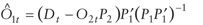 .
Therefore the objective function is .
Therefore the objective function is
![uppercase p hat superscript {uppercase m l s} equals minimum over uppercase p summation from lowercase t equals 1 to uppercase t [uppercase d subscript {lowercase t} minus [(uppercase d subscript {lowercase t} minus (uppercase o subscript {2 lowercase t} times uppercase p subscript {2})) times uppercase p superscript {'} subscript {1} times ((uppercase p subscript {1} times uppercase p superscript {'}) subscript {1}) superscript {-1} times uppercase p subscript {1} plus (uppercase o subscript {2 lowercase t} times uppercase p subscript {2}]] times [uppercase d subscript {lowercase t} minus [(uppercase d subscript {lowercase t} minus (uppercase o subscript {2 lowercase t} times uppercase p subscript {2})) times uppercase p superscript {'} subscript {1} times ((uppercase p subscript {1} times uppercase p superscript {'}) subscript {1}) superscript {-1} times uppercase p subscript {1} plus (uppercase o subscript {2 lowercase t} times uppercase p subscript {2}] superscript {'}](https://webarchive.library.unt.edu/eot2008/20081022194522im_/http://www.bts.gov/publications/journal_of_transportation_and_statistics/volume_05_number_23/images/gajequ20f.gif)
![equals minimum over uppercase p summation from lowercase t equals 1 to uppercase t [uppercase d subscript {lowercase t} times (uppercase i minus [uppercase p superscript {'} subscript {1} times ((uppercase p subscript {1} times uppercase p superscript {'} subscript {1}) superscript {-1}) times uppercase p subscript {1}] plus (uppercase o subscript {2 lowercase t} times uppercase p subscript {2}))] cross [uppercase d subscript {lowercase t} times (uppercase i minus [uppercase p superscript {'} subscript {1} times ((uppercase p subscript {1} times uppercase p superscript {'} subscript {1}) superscript {-1}) times uppercase p subscript {1}] plus (uppercase o subscript {2 lowercase t} times uppercase p subscript {2}))] superscript {'}](https://webarchive.library.unt.edu/eot2008/20081022194522im_/http://www.bts.gov/publications/journal_of_transportation_and_statistics/volume_05_number_23/images/gajequ20f_2.gif)
Estimates from this objective function produce a sequence that converges to the fixed but unknown true parameter (Gajewski 2000).
Remark: Confirmatory factor analysis occurs when all of the regressors are unknown resulting in P2 being empty. The objective function, similar to confirmatory factor analysis, is
 , ,
where
 . .
Ordinary least squares regression occurs when P1 is empty and
In most cases, model identifiability of the parameters holds because of the number of nonfeasible OD pairs. The biggest challenge is meeting the assumption
where  is full rank,
assuming is the matrix composed of the columns containing the assigned zeros in the kth row with those assigned zeros deleted. The nonfeasible OD pairs arise from the fact that a vehicle cannot have certain origin or destination combinations. Details of model identifiability and rank are found in Park et al. (2002). is full rank,
assuming is the matrix composed of the columns containing the assigned zeros in the kth row with those assigned zeros deleted. The nonfeasible OD pairs arise from the fact that a vehicle cannot have certain origin or destination combinations. Details of model identifiability and rank are found in Park et al. (2002).
Note that the LS method is used to demonstrate the approach, because the AVI data were found to
be well behaved. It should be noted that under the conditions presented in the theory section of
this paper  .
That is, as T goes to infinity the estimator under the mix model using least squares converges to the true split proportions (Gajewski 2000). .
That is, as T goes to infinity the estimator under the mix model using least squares converges to the true split proportions (Gajewski 2000).
A test of the imputation technique on data from the test bed was subsequently performed. It
was assumed that the volume from the first origin and the last origin are missing and the techniques
from confirmatory factor analysis were used to impute the missing origin volumes.
Table 3 shows the results, and it can be seen that the average percentage error for origins one and six are –30% and 3%, respectively. It can also be seen that the APE was lowest for the origin ramps that had the highest volume.
The important feature of the above technique is that it provides a consistent estimator for the split proportions despite missing a portion of the input information. While there are other imputation techniques (Chin et al. 1999; Gold et al. 2001), it is not clear if these techniques provide consistent estimators. Therefore, the above algorithm can be used when input information is missing or in situations where the input information is known a priori to be faulty. In this latter case, the faulty input volume would be removed prior to the estimation of the split
proportions.
Remark: The formulation derived in this paper was presented in OD format. Alternatively, in the data imputation format, the origins, O, can be treated as output parameters and the model
formulated as  This is a DO formulation where the split proportion Pkj represents the proportion of vehicles exiting at k and
entering at j.
This is a DO formulation where the split proportion Pkj represents the proportion of vehicles exiting at k and
entering at j.
The OD matrix was calculated for the full AVI data under both formulations. The OD matrix, under the DO formulation, was calculated using the LS estimator. The correlation between the OD matrix calculated from the DO model and the OD matrix calculated from the OD model is 0.9018; the correlation between the OD matrix calculated from the DO model and the true OD matrix is 0.9514; and the correlation between the OD matrix from the OD model and the true OD matrix is 0.9293. Therefore, the OD matrices from both formulations were approximately equal for
this test example.
CONCLUDING REMARKS
Origin-destination matrices are an integral component of off-line traffic models and real-time advanced traffic management centers. The recent deployment of ITS technology has resulted in the availability of a large amount of data that can be used to develop OD estimates. However, these data are subject to inaccuracies from a variety of sources. In this situation, the data may be “cleaned” and then used with existing OD estimators. Alternatively, OD estimators may be developed that are robust to the outliers characteristic of ITS data. This latter approach was the focus of this paper.
A robust estimator based on the L2E theory was first derived and compared with a traditional least squares estimator. In addition, closed-form asymptotic distributions for the variance were derived for both estimators. This is an important contribution because it allows variances, and therefore standard errors, to be calculated for the estimates. It was shown that while the L2E estimator was less efficient than the LS estimator, it was more statistically robust to bad data.
The models were applied to a corridor on Interstate 10 in Houston, Texas. The test bed was instrumented with AVI technology and therefore both AVI volumes and split proportions are available. This test bed provides a unique opportunity for comparing the estimators because an observed OD matrix is available, which is extremely rare for these types of studies. The asymptotic variance estimates were found to be slightly conservative as compared with the estimates derived using a bootstrap method. It was shown that while the LS and the L2E estimators had average mean absolute error ratios of approximately 50%, both replicated the observed OD at the 95% level of confidence. In addition, the accuracy of the estimates was highest for the OD pairs with higher relative volumes.
A Monte Carlo simulation was carried out to test the robustness of the techniques under different error types and error rates. It was found that the L2E estimator was much more robust than the LS estimator to outliers. However, after a certain threshold, which was 50% on the I-10 test network, the models were found to perform equally poorly. Lastly, a method for imputing missing origin data was developed and illustrated using the LS estimator.
It should be noted that the L2E approach is not limited to the input-output model used in this paper, but rather can be generalized to any number of OD problem formulations. For example, information from other detectors, such as those commonly found on main lanes, could also be added as a dependent variable and a consistent OD estimator could be formulated. In this way, the L2E estimator would be robust to malfunctions in any of the detectors. In addition, it was assumed in the model derivation that there was no prior information regarding the split proportion matrix. The model can also be generalized to incorporate prior information, which would help add “structure” to the over-parameterized model and could potentially reduce the percentage error of the estimates.
REFERENCES
Ashok, K. 1996. Estimation and Prediction of Time-Dependent Origin-Destination Flows, Ph.D. Dissertation. Massachusetts Institute of Technology, Cambridge, MA.
Basu, A., I. Harris, N. Hjort, and M. Jones. 1998. Robust and Efficient Estimation by Minimising a Density Power Divergence. Biometrika 85(3):549–59.
Bell, M.G.H. 1991. The Real Time Estimation of Origin-Destination Flows in the Presence of Platoon Dispersion. Transportation Research B 25(2/3):115–25.
Cascetta, E. 1984. Estimation of Trip Matrices from Traffic Counts and Survey Data: A Generalized Least Squares Estimator. Transportation Research B 22(4/5):289–99.
Cascetta, E. and S. Nguyen. 1988. A Unified Framework for Estimating or Updating Origin/Destination Matrices from Traffic Counts. Transportation Research B 22(6):437–55.
Chin, S., D.L. Greene, J. Hopson, H. Hwang, and B. Thompson. 1999. Towards National Indicators of VMT and Congestion Based on Real-Time Traffic Data. Paper presented at the 78th Annual Meetings of the Transportation Research Board, Washington, DC.
Davison, A. and D. Hinkley. 1997. Bootstrap Methods and Their Applications. New York, NY: Cambridge University Press.
Dixon, M. 2000. Incorporation of Automatic Vehicle Identification Data into the Synthetic OD Estimation Process, Ph.D. Thesis. Texas A&M University, College Station, TX.
Gajewski, B. 2000. Robust Multivariate Estimation and Variable Selection in Transportation and Environmental Engineering, Ph.D. Thesis. Texas A&M University, College Station, TX.
Gold, D.L., S.M. Turner, B.J. Gajewski, and C.H. Spiegelman. 2001. Imputing Missing Values in ITS Data Archives for Intervals Under Five Minutes. Paper presented at the 80th Annual Meetings of the Transportation Research Board, Washington, DC.
Hampel, F., E. Ronchetti, P. Rousseeuw, and A. Werner. 1986. Robust Statistics: The Approach Based on Influence Functions. New York, NY: John Wiley and Sons.
Huber, P. 1981. Robust Statistics. New York, NY: John Wiley and Sons.
Maher, M.J. 1983. Inference on Trip Matrices from Observations on Link Volumes: A Bayesian Statistical Approach. Transportation Research B 17(6):435–47.
McNeil, S. and C. Henderickson. 1985. A Regression Formulation of the Matrix Estimation Problem. Transportation Science 19(3):278–92.
Nihan, N.L. and M.M. Hamed. 1992. Fixed Point Approach to Estimating Freeway Origin-Destination Matrices and the Effect of Erroneous Data on Estimate Precision. Transportation Research Record 1357:18–28.
Park, E.S., C.H. Spiegelman, and R.C. Henry. 2002. Bilinear Estimation of Pollution Source Profiles and Amounts by using Multivariate Receptor Models (with discussions). Environmetrics 13:775–98.
Robillard, P. 1975. Estimating the OD Matrix from Observed Link Volumes. Transportation Research 9:123–28.
Scott, D.W. 1999. Parametric Modeling by Minimum L2 Error, Technical Report 98-3. Department of Statistics, Rice University, Houston TX.
Sherali, H.D., N. Arora, and A.G. Hobeika. 1997. Parameter Optimization Methods for Estimating Dynamic Origin-Destination Trip-Tables. Transportation Research B 31(2):141–57.
Terrell, G.R. 1990. The Maximal Smoothing Principle in Density Estimation. Journal of the American Statistical Association 85:470–7.
Turner, S., L. Albert, B. Gajewski, and W. Eisele. 1999. Archived ITS Data Archiving: Preliminary Analyses of San Antonio TransGuide Data. Transportation Research Record 1719:85–93.
Van Zuylen, H. 1980. The Most Likely Trip Matrix Estimation from Traffic Counts. Transportation Research B 16(3):281–93.
APPENDIX
Notation
The following notation serves as a reference guide throughout this paper:
T Number of time periods. Each time period is of
duration t.
p Number of destinations in the system.
q Number of origins in the system.
r Number of nonfeasible elements of P.
O Matrix of observed volumes from q origins over T time periods (T by q).
D Matrix of observed volumes from p destinations over T time periods (T by p).
Ot Row vector of observed volumes from q origins from the tth row, t
= 1,2,3,…,T.
Dt Row vector of observed volumes from p destinations from the tth row, t = 1,2,3,…,T.
Otk Element (t,k) of the matrix O,
t = 1,2,3,…,T; k = 1,2,3,…, q.
P Split proportion matrix between q origins and p destinations (q by p).
Pkj Proportion of vehicles that enter at origin k and exit at destination ramp j where k = 1,2,3,…,q, and
j = 1,2,3,…,p.
Pj Column vector of q split proportions from the jth destination,
j = 1,2,3,…, p.
Matrix of random errors with n rows and p columns.
Av Vectorization of matrix A. The operator Av takes the columns of A and stacks them on top of each other.
For example,
 Stacked
version of . Stacked
version of .
 Row vector of
p elements from the tth
row of , t = 1,2,3,…,T. Row vector of
p elements from the tth
row of , t = 1,2,3,…,T.
Pv Stacked version of P.
M Matrix that maps the elements of Pv that are nonfeasible to zero. M is of size r X qp.
Ov Stacked version of the matrix O.
 Kronecker
product Kronecker
product  . .
X* The regressors used in the stacked
model, , X* is
Tp X qp.
G Equality constraint matrix.
G = [G1G2] Partition of G into matrices G1 and G2, where rank(G) = rank(G1)
= q + r, and G1 is (q + r) X (q + r).
G2 is (q + r) X (pq–q–r)
Note that G is permuted until G1 is full rank.
G1 The nonsingular portion of the constraint matrix G.
G2 The “left over” portion of the constraint matrix G.
![uppercase p superscript {v} equals [2 by 1 matrix where (row 1 column 1 is uppercase p superscript {lowercase v} subscript {1}) and (row 2 column 1 is uppercase p superscript {lowercase v} subscript {2}]](https://webarchive.library.unt.edu/eot2008/20081022194522im_/http://www.bts.gov/publications/journal_of_transportation_and_statistics/volume_05_number_23/images/gajapp10.gif) Partition
of Pv such that the elements correspond to [G1G2].
The size of Partition
of Pv such that the elements correspond to [G1G2].
The size of
 and and
 are r + q and pq–r–q, respectively. are r + q and pq–r–q, respectively.
The portion of Pv that corresponds to G1.
The portion of Pv that corresponds to G2.
Partition
of X* such that the elements correspond to [G1G2].
1q Column vector of q ones.
0r Column vector of r zeros.
g GPv = g,
where
 Variance
for each row of . Variance
for each row of .
Y2  (Tp X 1). (Tp X 1).
Y2t The tth element of Y2.
W2 
(Tp X (pq–q–r)).
W2t The tth row vector of W2.
Z Z = Yr /  . (Tp X 1). . (Tp X 1).
Zt The tth element of Z.
U  (Tp X (pq–q–r)). (Tp X (pq–q–r)).
Ut The tth row vector of U.
W2tk The (t,k) element of W2.
(Tp 3 1).
 Estimated
vector of Estimated
vector of  using least squares. using least squares.
 Estimated
vector of using L2E. Estimated
vector of using L2E.
 Influence function (see Hampel et al. 1986). Influence function (see Hampel et al. 1986).
 Normal
distribution with mean Normal
distribution with mean  and variance and variance
 . .
Detail Theory
Step 1
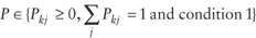
Condition 1. The split proportions (P) are positive for all feasible origin and destination combinations and equal to zero for all nonfeasible combinations.
Therefore the general model is written algebraically as follows:
and
The detailed derivation of the L2E objective function is
![minimum over uppercase p uppercase f subscript {uppercase l subscript {2} uppercase e} equals minimum over uppercase p {the integral from negative infinity to positive infinity [lowercase f (uppercase d subscript {lowercase t j} vertical bar uppercase o subscript {lowercase t} times uppercase p subscript {lowercase j}) minus lowercase f (uppercase d subscript {lowercase t j} vertical bar uppercase o subscript {lowercase t} times uppercase p subscript {0})] superscript {2} times lowercase d times uppercase d subscript {lowercase t j}}](https://webarchive.library.unt.edu/eot2008/20081022194522im_/http://www.bts.gov/publications/journal_of_transportation_and_statistics/volume_05_number_23/images/gajequ3.gif)
![equals minimum over uppercase p {integral from negative infinity to positive infinity lowercase f superscript {2} (uppercase d subscript {lowercase t j} vertical bar uppercase o subscript {lowercase t} times uppercase p subscript {lowercase j}) times lowercase d times uppercase d subscript {lowercase t j} minus 2 times uppercase e [uppercase f (uppercase d subscript {lowercase t j} vertical bar uppercase o subscript {lowercase t} times uppercase p subscript {lowercase j})] plus the integral from negative infinity to positive infinity lowercase f superscript {2} times (uppercase d subscript {lowercase t j} vertical bar uppercase o subscript {lowercase t} times uppercase p subscript {lowercase {0}) lowercase d times uppercase d subscript {lowercase t j}}](https://webarchive.library.unt.edu/eot2008/20081022194522im_/http://www.bts.gov/publications/journal_of_transportation_and_statistics/volume_05_number_23/images/gajequ3_2.gif)
![approximately equals minimum over uppercase p {integral from negative infinity to positive infinity [lowercase f times (uppercase d subscript {lowercase t j} vertical bar uppercase o subscript {lowercase t} times uppercase p subscript {lowercase j})] superscript {2} times lowercase d times uppercase d subscript {lowercase t j} minus 2 divided by uppercase t times lowercase p summation from lowercase t equals 1 to uppercase t summation from lowercase j equals 1 to lowercase p times lowercase f (uppercase d subscript {lowercase t j} vertical bar uppercase o subscript {lowercase t} times uppercase p subscript {lowercase j})}.](https://webarchive.library.unt.edu/eot2008/20081022194522im_/http://www.bts.gov/publications/journal_of_transportation_and_statistics/volume_05_number_23/images/gajequ3_3.gif)
Because the third component in the second line of equation A1 does not have the optimization parameter P (but only the true parameter P0), it can be taken as a constant and ignored during optimization. The empirical density function is used to estimate the expectation in the second line of equation A1 (Scott 1999).
Details of the following results appear in Gajewski (2000). The error structure for the reduced problem is shown in equation A2.
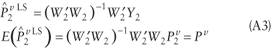
Therefore, equation A3 provides the estimate of the reduced regression parameters under LS, and it can be seen that it is unbiased.
The variance of this estimate is shown in equation A4.
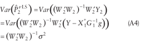
Note that equations A3 and A4 are based on the assumption that W2 is full rank. Lemma 1 relates the rank of the origins, O, to that of the rank of W2.
Lemma 1: If O is full rank, then W2 is full rank. (See Gajewski (2000) for proof.)
Note that it is assumed that there will be multiple days’ worth of data and multiple time periods in each day. Therefore, the variation of volume between days and within days causes O to be full rank and therefore W2 is full rank.
Similar to the variance of the estimates in equation A4, the variance estimates
for  are presented in equations A5 and A6. are presented in equations A5 and A6.
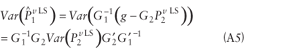
The covariance between the
estimates  and are shown in equation A6.
Notice that the reparameterization causes the problem to be unconstrained except for
the non-negativity constraints. When deriving the asymptotic distributions of the
estimators ,
it is assumed to be in the interior of the parameter space. From a physical viewpoint, this means that the true split proportion over the long term would never lie on the boundary (i.e., be equal to zero) for a feasible OD pair. It is assumed that this assumption is valid on the highway networks where most ITS traffic monitoring devices are located. In addition, if this assumption is violated, the origins and destinations can be combined to alleviate the problem. Regardless, this assumption will need to be checked when applying the model.
The asymptotic distributions for the two estimation methods are derived using properties of
M-estimators (Huber 1981). Equation A7 shows the L2E model. As
discussed, is
estimated prior to using equation A7. Let N(A,B2) be the normal
probability density function with a mean of A and variance B2, then
![arg minimum over uppercase p uppercase f subscript {uppercase l subscript {2} uppercase e} equals arg minimum over uppercase p [1 divided by (2 times the square root {lowercase pi} times lowercase sigma) minus (2 divided by (uppercase t times lowercase p)) summation from lowercase t equals 1 to uppercase t summation from lowercase j equals 1 to lowercase p uppercase n (uppercase d subscript {lowercase t j} minus (uppercase o subscript {lowercase t} times uppercase p subscript {lowercase j}), lowercase sigma superscript {2})] equals arg minimum over uppercase p [negative 2 divided by (uppercase t times lowercase p) summation from lowercase t equals 1 to uppercase t summation from lowercase j equals 1 to lowercase p uppercase n (uppercase d subscript {lowercase t j} minus (uppercase o subscript {lowercase t} times uppercase p subscript {lowercase j}), lowercase sigma superscript {2})]](https://webarchive.library.unt.edu/eot2008/20081022194522im_/http://www.bts.gov/publications/journal_of_transportation_and_statistics/volume_05_number_23/images/gajequ13.gif)
with
A reparameterized model may be obtained by using the variance to standardize the model.
Let  and . Therefore,
the reparameterized reduced model will
be
and . Therefore,
the reparameterized reduced model will
be 
 where and the objective function, is shown below:
Because the L2E is an M-estimator, the distribution properties are straightforward to derive and will be useful in the derivations of the distribution.
Definition 1: (Huber 1981): For a
sample x1,x2,...,xT from the sample
space F, the M-estimate corresponding
to  is the “statistical function”
 , that
is, a solution VT of the equation: , that
is, a solution VT of the equation:
The L2E estimator is an M-estimator because of a calculation of the derivative of the objective function.
Property 1:  is an M-estimator (see Gajewski (2000) for proof). is an M-estimator (see Gajewski (2000) for proof).
Huber (1981, p. 165) proves the asymptotic properties for the reduced model of the
form  .
Note that this proof assumes .
Note that this proof assumes  and the three regularity conditions, referred to as RC1 to RC3, are met.
Property 2: Regularity conditions RC1 to RC3 hold for the OD problem (see Gajewski (2000) for proof).
Theorem 1 shows the distribution of the LS estimator in a linear model setting is asymptotic normal.
Theorem 1: (Huber 1981, p. 159):
If  , then all
the LS estimates , then all
the LS estimates 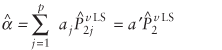 are asymptotically normal. are asymptotically normal.
Theorem 1 states that asymptotic normality holds for both objective functions in this paper. Therefore, the identification of the mean and variance define the asymptotic distribution.
Using Theorem 1, the LS variance is calculated as shown in equation A10.
Similarly, the variance for the L2E is shown in equation A11.
![var (uppercase p hat superscript {lowercase v times uppercase l subscript {2} uppercase e} subscript {2}) equals (uppercase e [lowercase psi superscript {2}]) divided by ((uppercase e [lowercase psi superscript {'}]) superscript {2}) times ((uppercase u superscript {'} times uppercase u) superscript {-1})](https://webarchive.library.unt.edu/eot2008/20081022194522im_/http://www.bts.gov/publications/journal_of_transportation_and_statistics/volume_05_number_23/images/gajequ17.gif)
Note that, in order to use equation A11, the errors need to be identified. For example, if it is assumed that the error distribution is normal, Property 3 shows the exact value of the
ratio ![(uppercase e [lowercase psi superscript {2}]) divided by ((uppercase e [lowercase psi superscript {'}]) superscript {2})](https://webarchive.library.unt.edu/eot2008/20081022194522im_/http://www.bts.gov/publications/journal_of_transportation_and_statistics/volume_05_number_23/images/gajequ17b.gif) . .
Property 3:
Suppose 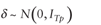 , then , then
![a) uppercase e [lowercase psi superscript {2}] equals 1 divided by (3 times the square root {3}) times (uppercase e (uppercase psi superscript {2})) equals 1 divided by (3 times the square root 3).](https://webarchive.library.unt.edu/eot2008/20081022194522im_/http://www.bts.gov/publications/journal_of_transportation_and_statistics/volume_05_number_23/images/gajequ17c.gif)
![b) uppercase e [lowercase psi superscript {'}] equals 1 divided by (2 times the square root {2})](https://webarchive.library.unt.edu/eot2008/20081022194522im_/http://www.bts.gov/publications/journal_of_transportation_and_statistics/volume_05_number_23/images/gajequ17d.gif)
and therefore ![(uppercase e [lowercase psi superscript {2}]) divided by ((uppercase e [lowercase psi superscript {'}]) superscript {2}) equals 8 divided by (3 times the square root {3})](https://webarchive.library.unt.edu/eot2008/20081022194522im_/http://www.bts.gov/publications/journal_of_transportation_and_statistics/volume_05_number_23/images/gajequ17e.gif)
(See Gajewski (2000) for proof.)
If the error distribution is non-normal then an approximation is used, as shown in the Remark.
Remark: The nonparametric estimation of the above equation is:
![uppercase e [lowercase psi superscript {2}] divided by (uppercase e [lowercase psi superscript {'}]) superscript {2} equals summation from lowercase t equals 1 to uppercase t (lowercase psi superscript {2} subscript {lowercase i} divided by uppercase t) divided by (summation from lowercase t equals 1 to uppercase t lowercase psi superscript {'} subscript {lowercase i} divided by uppercase t) subscript {2} equals uppercase t times (summation from lowercase t equals 1 to uppercase t times lowercase psi superscript {2} subscript {lowercase i}) divided by ((summation from lowercase t equals 1 to uppercase t lowercase psi superscript {'} subscript {lowercase i}) subscript {2})](https://webarchive.library.unt.edu/eot2008/20081022194522im_/http://www.bts.gov/publications/journal_of_transportation_and_statistics/volume_05_number_23/images/gajequ17f.gif)
(See Gajewski (2000) for proof.)
The asymptotic distributions are stated in Corollary 1 for completeness.
Corollary 1: Let a be a fixed vector. Under the conditions of the above models and the regularity conditions RC1–RC3, equations A12 and A13 are the asymptotic distributions for the LS and L2E objective functions,
respectively:
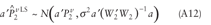
![lowercase a superscript {'} times uppercase p hat superscript {lowercase v times uppercase l subscript {2} times uppercase e} subscript {2} ~ uppercase n times (lowercase a superscript {'} times uppercase p superscript {lowercase v} subscript {2}, lowercase sigma superscript {2} times lowercase a superscript {'} times (uppercase e [lowercase psi superscript {2}]) divided by ((uppercase e times [lowercase psi superscript {'}]) superscript {2}) times (uppercase w superscript {'} subscript {2} times uppercase w subscript {2}) subscript {-1} times lowercase a)](https://webarchive.library.unt.edu/eot2008/20081022194522im_/http://www.bts.gov/publications/journal_of_transportation_and_statistics/volume_05_number_23/images/gajequ19.gif)
(See Gajewski (2000) for proof.)
Based on the distributional properties shown in Corollary 1, the L2E method is less efficient than the LS method as shown in Corollary 2.
Corollary 2:
When  , then for every b (fixed vector), , then for every b (fixed vector),
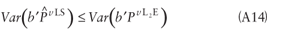
(See Gajewski (2000) for proof.)
Note that the nonparametric formula shown in the Remark is preferred when the parametric distribution of the error is not known.
Address for Correspondence and End Notes
Byron Gajewski, Schools of Allied Health and Nursing, 3024 SON, University of Kansas Medical Center, 3901 Rainbow Blvd., Kansas City, KS 66160.
Email: Bgajewski@kumc.edu.
1 Basu et al. (1998) and Scott (1999) contributed the idea to the parametric literature. L2 refers to the squared distance between two points. The L2E was originally used in kernel density estimation (see, e.g., Terrell 1990).
2 See Dixon (2000) for specific data extraction techniques.
|