U.S. Bureau of Labor Statistics

Compensation and Working Conditions Online

Pay Relatives for Major Metropolitan Areas
by Parastou Karen Shahpoori
Bureau of Labor Statistics

Originally Posted: April 28, 2003
Revision posted: June 16, 2004

To facilitate pay comparisons among major metropolitan areas, the Bureau of Labor Statistics has developed pay relatives, or ratios of pay, for nine groups of occupations (as well as for all occupations combined) in each of 77 metropolitan areas.

How do the earnings of workers in San Francisco or Houston compare with those of workers in the United States overall? The National Compensation Survey (NCS), which was introduced in 1997, collects earnings and other data on employee compensation covering 480 detailed occupations in 154 metropolitan and nonmetropolitan areas. Occupational earnings from the NCS are published annually for more than 80 metropolitan areas and for the United States as a whole.¹

These estimates are produced by surveying a randomly selected sample of occupations. In the NCS, samples of employer establishments and occupations are selected using a "probability proportionate to size" technique. All establishments and occupations in the survey are assigned a weight to reflect the probability of their selection in the sample. These weights reflect the relative size of the occupation within the establishment and the relative size of the establishment within the sample universe. Occupations that are relatively rare will have less opportunity to contribute to the pay relatives because their chance of selection in the sample is less than more common occupations.

In order to facilitate comparisons of occupation pay levels across metropolitan areas, BLS has developed pay relatives, or ratios of pay, for nine groups of occupations (as well as for all occupations) in each of 77 major metropolitan areas and the United States as a whole.

The pay relative for each occupational group in an area expresses its average pay² as a percent of the pay for a comparable occupation group in the entire United States. The pay relative for the United States as whole always equals 100. For example, the pay relative for all occupations in San Francisco was 119 in 1998, meaning that workers in San Francisco earned 19 percent more than the U.S. average for comparable workers. The pay relative for Houston was 104, or 4 percent more than the U.S. average. The pay relatives for each area are expressed in terms of their relation to the U.S. average.

The nine occupation groups used in pay relatives are (1) professional specialty and technical occupations; (2) executive, administrative, and managerial occupations; (3) sales occupations; (4) administrative support occupations, including clerical; (5) precision production, craft, and repair occupations; (6) machine operators, assemblers, and inspectors; (7) transportation and material moving occupations; (8) handlers, equipment cleaners, helpers, and laborers; and (9) service occupations. Table 1 presents 1998 pay relatives for each occupational group in 77 metropolitan areas.

Comparability

There are a number of occupational characteristics that the National Compensation Survey captures that can influence pay levels, including the mix of occupations and work levels studied, differing workweeks, and survey timing. Since the survey design calls for "probability proportionate to size" occupational sampling, the occupations selected in one area will not be the same as those selected in another area. In addition, occupational work levels as well as scheduled hours per week will differ between areas. Data for each NCS area are published once per year, but the publications are produced in "panels" every 3 months. Thus, the published average reference dates will usually differ between areas. When calculating pay relatives BLS tries to decrease the effect of these different factors as much as possible. Occupations, levels, workweeks, and reference dates are taken into account in the computation of pay relatives.

Occupations and levels. The pay relative calculation for each area uses comparable jobs at both the area and national levels. That is, occupations found in the national database that are not found in the area database are not used in the calculation of pay relatives for that area. For example, if architects are not found in the Denver survey, then national data for architects are not used in the calculation of pay relatives for Denver.

Similarly, the working "levels" of incumbents within occupations are also comparable between the area and the national database when calculating pay relatives. These levels reflect knowledge, skills, responsibility, and other factors.³ Levels not observed within an area’s occupations are not used in the national database for calculating pay relatives. For example, if the category level-13 architects is not found in the Denver survey, then level-13 architects are removed from the national estimates and are not used in the calculation of pay relatives for Denver.

Hours adjustment. In the National Compensation Survey, average rates of pay are weighted by the average number of annual hours worked (and by the number of employees). That is, rates of pay associated with fewer annual hours will not count as much in the average as rates associated with greater annual hours. The hourly wages of full-time workers count more than those of part-time workers.

When determining how area earnings compare with national earnings, the average rates of pay calculated for comparable occupations within the nine occupation groups reflect a comparable composition of occupation annual hours. In order to maintain comparable annual hours, the total annual hours of work calculated for each occupation in the national database are also used in the area calculation of average hourly rates of pay for pay relative purposes.

Reference month adjustment. In the National Compensation Survey, data for each area are collected once per year. The reference date for each area differs depending on when the data were collected. For example, the data used to produce the 1998 estimates for the United States as a whole were compiled from data collected from the 154 NCS localities between July 1997 and April 1999. The average reference date for these 154 areas in the United States was August 1998. Before calculating the pay relatives for each area, an adjustment was made to the U.S. wage rate to account for differences between the average reference month for each area and the reference month of August 1998 for the United States as a whole. This adjustment was based on published estimates of wage change from the Employment Cost Index (ECI).

To calculate the adjustment factor, monthly indexes of wages were interpolated⁴ from the published ECI quarterly indexes for all occupations and for each of the region occupation groups. The cumulative change in the wage index between August 1998 and the reference month for a specific area was used to adjust the national wage estimate. The adjusted national wage estimate was used to calculate the pay relative for the area. For example, to adjust the national estimate of comparable wages to reflect Denver’s May reference month, the interpolated wage index for all occupations in May is divided by the interpolated index for August to estimate wage change over the period. This estimate of change is the adjustment, or ECI factor, applied to the national estimate of comparable average wages. That is, national average comparable wages are decreased to reflect what they would have been in May. This adjusted estimate is used to calculate the pay relative for Denver and for any area with a May reference month.

Comparing wages in four cities

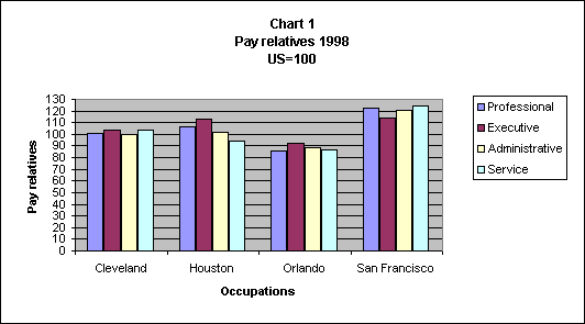
Chart 1 compares four of the nine major occupational groups⁵--professional specialty; executive; administrative support, including clerical; and service occupations--from four different metropolitan areas of the United States: Cleveland-Akron, Ohio; Houston-Galveston-Brazoria, Texas; Orlando, Florida; and San Francisco-Oakland-San Jose, California. As shown in chart, earnings in San Francisco were much higher than the national average for all four occupational groups. (The overall U.S. rate equals 100.) In Orlando, Florida, on the other hand, the pay relatives for all four occupational groups were below the U.S. average.⁶

Differences between the NCS and earlier surveys

The locality wage data produced from the National Compensation Survey differ considerably from those of the survey’s predecessor--the Occupational Compensation Survey.⁷ For example, the NCS covers all workers and provides information on a much broader range of occupations. Occupations surveyed for the NCS are selected using probability techniques from a list of all occupations present in each establishment. The NCS classification system specifies up to 480 individual occupations. Data from the Occupational Compensation Survey, on the other hand, were limited to a preselected list of 38 occupations, which represented only a small subset of all occupations in the economy. Moreover, the former survey did not use occupational sampling within an establishment.

In the Occupational Compensation Survey, pay relatives were calculated, but only when the data collected for preselected occupations were judged sufficiently representative of all occupations in the area. The NCS is designed to collect a representative sample of occupations in each area, and the calculated pay relatives reflect this. Furthermore, the former survey collected data for full-time workers only, while the NCS collects data for both full- and part-time workers.

Limitations

Pay relatives derived from the National Compensation Survey have certain limitations. For example, they do not take into account some wage determinants. There are many commonly recognized determinants of wages, including the effects on average wage rates from different methods of pay (time versus incentive), collective bargaining status (union versus nonunion), establishment size, and industry. The sample sizes in the NCS area survey are too small to permit estimate pay relatives for each of these determinants.

Another limitation of pay relatives produced from the National Compensation Survey is that the pay relatives for two different areas are not strictly comparable. To make precise pay relative comparisons, the mix of occupations and work levels studied, the differing workweeks, and the average reference periods would need to be adjusted. Currently, such adjustments are made between each area and the United States as a whole. To compare each area to every other area would require thousands of additional calculations.

Finally, pay relatives from the National Compensation Survey do not address nonwage compensation. For example, an architect in Denver may earn $25 per hour and have a health care benefit worth an additional $3 per hour, while an architect in Houston earning similar pay might not receive a health care benefit. The pay relative only includes the wage compensation.

Parastou Karen Shahpoori
Economist, Division of Compensation Data Estimation, Bureau of Labor Statistics.
Telephone: (202) 691-6290, E-mail: Shahpoori_K@bls.gov

NOTE: This is a revised version of an article that was originally published in April 2003. This version corrects the description about how work schedules affect the pay comparisons by indicating that annual hours, rather than weekly hours, are used. This version also revises the last sentence of the second paragraph to clarify how the relative size of occupations affects the pay relatives calculations. None of the data tables have been changed.

Notes

1 The data used in this article are from 1998, the most recent data available when the article was completed. See National Compensation Survey: Occupational Wages in the United States, 1998, Bulletin 2529 (Bureau of Labor Statistics, September 2000). For more information, see the National Compensation Survey (NCS) website on the Internet at http://www.bls.gov/ncs/home.htm.

2 Hourly wages are defined as the straight-time earnings paid to employees before deductions of any type. They exclude premium pay for overtime, nonproduction bonuses, and tips. Average hourly wages also reflect the hours worked by surveyed occupations.

3 See Appendix C in National Compensation Survey: Occupational Wages in the United States, 1998, Bulletin 2529, for a complete description of the leveling criteria.

4 Because the ECI is published quarterly (December, May, June and September), the estimates for the months in between have to be interpolated to relate to the reference month of the area estimates.

5 For the complete list of occupations included in each major occupational group, see Appendix B in National Compensation Survey: Occupational Wages in the United States, 1998, Bulletin 2529.

6 See table 1 for a complete listing of pay relatives for 77 major metropolitan areas.

7 Occupation Compensation Survey data were last published in Occupational Compensation Survey: National Summary, 1996, Bulletin 2497 (Bureau of Labor Statistics, March 1998).

Table 1. Pay relatives for major occupational groups in metropolitan areas, National Compensation Survey, 1998 (For each occupational group, average pay for all industries = 100)
Metropolitan area	Total	White collar(1)				Blue collar(1)				Service
Metropolitan area	Total	Professional	Executive	Sales	Administrative	Precision	Machine operators	Transportation	Handlers	Service
United States(2)	100	100	100	100	100	100	100	100	100	100
Amarillo, TX	87	84	89	96	83	92	82	83	92	84
Anchorage, AK	110	105	109	111	111	123	101	102	119	116
Atlanta, GA	99	99	103	99	101	96	98	96	101	95
Augusta-Aiken, GA-SC	94	95	102	93	96	92	98	87	94	85
Austin-San Marcos, TX	93	90	96	109	93	96	82	93	95	95
Birmingham, AL	94	89	106	91	92	93	96	79	96	93
Bloomington, IN	91	91	95	88	91	90	--	81	92	88
Bloomington-Normal, IL	104	93	--	95	92	102	117	131	106	106
Boston-Worcester-Lawrence, MA-NH-ME-CT	104	105	98	101	108	103	95	108	108	112
Brownsville-Harlingen-San Benito, TX	82	90	86	87	78	77	71	78	72	80
Buffalo-Niagra Falls, NY	100	97	97	90	101	103	107	102	106	107
Charleston-North Charleston, SC	87	91	88	81	86	81	82	84	87	87
Charlotte-Gastonia-Rock Hill-High Point, NC-SC	94	88	98	103	97	93	99	97	98	92
Chicago-Gary-Kenosha, IL-IN-WI	107	102	103	105	109	112	114	117	117	110
Cincinnati-Hamilton, OH-KY-IN	95	92	95	95	94	93	94	99	103	99
Cleveland-Akron, OH	103	101	104	105	100	103	107	109	108	104
Columbus, OH	96	94	92	93	98	100	95	96	104	101
Corpus Christi, TX	89	89	111	96	82	90	93	75	82	82
Dallas-Fort Worth, TX	95	94	99	91	98	93	93	95	95	93
Dayton-Springfield, OH	96	94	91	95	93	101	109	102	100	101
Denver-Boulder-Greeley, CO	97	96	99	97	99	93	87	93	102	102
Detroit-Ann Arbor-Flint, MI	110	110	104	107	108	112	121	116	123	106
Elkhart-Goshen, IN	99	99	96	88	98	97	104	112	107	97
Fort Collins-Loveland, CO	88	92	85	98	86	86	80	85	84	91
Grand Rapids-Muskegon-Holland, MI	103	107	98	107	97	103	111	97	103	106
Greensboro-Winston-Salem, NC	97	93	102	106	97	93	95	96	99	95
Greenville, SC	93	90	97	99	94	91	92	89	98	90
Hartford, CT	109	115	99	106	110	103	100	106	107	119
Honolulu, HI	107	104	103	105	109	115	110	97	105	111
Houston-Galveston-Brazoria, TX	104	106	113	100	102	104	99	94	97	94
Huntsville, AL	95	97	101	93	92	91	102	84	92	87
Indianapolis, IN	99	97	98	106	97	104	103	103	104	98
Iowa City, IA	92	90	95	88	93	88	96	82	91	95
Johnstown, PA	89	93	91	82	86	83	85	82	89	97
Kalamazoo-Battle Creek, MI	101	99	97	96	102	100	106	100	113	104
Kansas City, MO-KS	93	93	88	85	92	97	105	100	103	95
Knoxville, TN	90	91	97	86	87	89	91	81	97	87
Lincoln, NE	88	86	88	85	85	87	89	90	97	91
Los Angeles-Riverside-Orange County, CA	107	111	111	116	108	104	89	93	96	108
Louisville, KY-IN	99	101	97	97	95	101	107	93	101	95
Melbourne-Titusville-Palm Bay, FL	86	85	92	82	86	92	80	84	85	85
Memphis, TN-AR-MS	95	91	100	111	94	95	98	93	98	90
Miami-Fort Lauderdale, FL	96	95	102	103	97	94	84	99	95	95
Milwaukee-Racine, WI	99	94	95	89	100	102	107	108	108	103
Minneapolis-St. Paul, MN-WI	104	99	97	107	106	106	115	114	114	112
Mobile, AL	89	90	92	96	84	92	90	82	97	86
New Orleans, LA	94	99	104	94	89	93	87	88	88	88
New York-Northern New Jersey-Long Island, NY-NJ-CT-PA	116	120	116	110	117	113	98	111	117	122
Norfolk-Virginia Beach-Newport News, VA-NC	90	89	99	91	90	89	96	77	82	87
Oklahoma City, OK	92	88	95	97	88	93	103	103	91	85
Orlando, FL	88	86	92	91	89	89	84	80	88	87
Philadelphia-Wilmington-Atlantic City, PA-NJ-DE-MD	108	109	102	111	108	104	109	108	117	109
Phoenix-Mesa, AZ	96	95	102	110	96	100	88	89	86	95
Pittsburgh, PA	100	101	99	89	100	98	99	100	110	103
Portland-Salem, OR-WA	101	99	98	99	102	104	98	104	102	112
Providence-Fall River-Warwick, RI-MA	103	108	102	97	107	97	92	107	93	106
Raleigh-Durham-Chapel Hill, NC	95	91	100	97	96	92	100	97	94	94
Reading, PA	100	108	91	89	96	96	101	94	105	111
Reno, NV	95	96	87	107	97	101	86	96	91	98
Richland-Kennewick-Pasco, WA	99	94	99	89	103	104	92	110	92	105
Richmond-Petersburg, VA	93	92	96	89	94	96	96	87	97	90
Rochester, NY	102	105	101	91	97	97	96	98	107	114
Rockford, IL	96	92	97	95	93	99	106	102	105	95
Sacramento-Yolo, CA	105	103	101	120	105	107	99	107	106	107
Salinas, CA	108	110	104	121	101	111	100	108	107	113
San Antonio, TX	92	94	104	96	90	85	86	75	84	90
San Diego, CA	100	105	99	101	104	97	83	95	94	102
San Francisco-Oakland-San Jose, CA	119	122	114	111	121	118	100	116	119	124
Seattle-Tacoma-Bremerton, WA	105	105	96	105	106	107	105	108	104	112
Springfield, MA	105	104	103	95	106	94	113	105	103	114
Springfield, MO	88	87	91	91	81	89	94	92	92	87
St. Louis, MO-IL	96	94	95	99	93	99	100	96	109	96
Tallahassee, FL	81	81	84	82	81	78	83	72	77	83
Tampa-St. Petersburg-Clearwater, FL	90	89	96	94	89	87	81	84	85	89
Visalia-Tulare-Porterville, CA	97	105	98	97	93	89	90	88	92	103
Washington-Baltimore, DC-MD-VA-WV	103	102	101	101	105	103	106	102	111	103
Youngstown-Warren, OH	98	96	101	100	93	98	106	99	99	101
Footnotes: (1) The full titles for the major occupational groups under the white-collar category are professional specialty and technical; executive, administrative, and managerial; sales; and administrative support, including clerical. The full titles for the groups under the blue-collar category are precision production, craft, and repair; machine operators, assemblers, and inspectors; transportation and material moving; and handlers, equipment cleaners, helpers, and laborers. (2) This survey covers all 50 States. Collection was conducted between July 1997 and April 1999. The average reference period was August 1998.
NOTE: Dashes indicate that no data were reported or that data did not meet publication criteria.

Chart 1. Pay relatives 1998

Chart 1. Pay relatives, 1998
	Cleveland	Houston	Orlando	San Francisco
Professional	101	106	86	122
Executive	104	113	92	114
Administrative	100	102	89	121
Service	104	94	87	124