
|
||
|
|
||
Oxygen is one of the most significant keys to deciphering past climates. Oxygen comes in heavy and light varieties, or isotopes, which are useful for paleoclimate research. Like all elements, oxygen is made up of a nucleus of protons and neutrons, surrounded by a cloud of electrons. All oxygen atoms have 8 protons, but the nucleus might contain 8, 9, or 10 neutrons. “Light” oxygen-16, with 8 protons and 8 neutrons, is the most common isotope found in nature, followed by much lesser amounts of “heavy” oxygen-18, with 8 protons and 10 neutrons. |
| ||

The ratio (relative amount) of these two types of oxygen in water changes with the climate. By determining how the ratio of heavy and light oxygen in marine sediments, ice cores, or fossils is different from a universally accepted standard, scientists can learn something about climate changes that have occurred in the past. The standard scientists use for comparison is based on the ratio of oxygen isotopes in ocean water at a depth of 200-500 meters. What climate factors influence the ratio of oxygen isotopes in ocean water?Evaporation and condensation are the two processes that most influence the ratio of heavy oxygen to light oxygen in the oceans. Water molecules are made up of two hydrogen atoms and one oxygen atom. Water molecules containing light oxygen evaporate slightly more readily than water molecules containing a heavy oxygen atom. At the same time, water vapor molecules containing the heavy variety of oxygen condense more readily. |
The Oxygen-18 isotope has an extra two neutrons, for a total of 10 neutrons and 8 protons, compared to the 8 neutrons and 8 protons in a normal oxygen atom. The slighty greater mass of 18O—12.5 percent more than 16O—results in differentiation of the isotopes in the Earth’s atmosphere and hydrosphere. Scientists measure differences in oxygen isotope concentrations to reveal past climates. [Roll mouse over nuclei to animate.] (Illustration by Robert Simmon, NASA GSFC) | ||
 |

Cooler air can hold less moisture than warmer air, so as air cools by rising into the atmosphere or moving toward the poles, moisture begins to condense and fall as precipitation. At first, the rain contains a higher ratio of water made of heavy oxygen, since those molecules condense more easily than water vapor containing light oxygen. The remaining moisture in the air becomes depleted of heavy oxygen as the air continues to move poleward into colder regions. As the moisture reaches the upper latitudes, the falling rain or snow is made up of more and more water molecules containing light oxygen. Ocean waters rich in heavy oxygen: During ice ages, cooler temperatures extend toward the equator, so the water vapor containing heavy oxygen rains out of the atmosphere at even lower latitudes than it does under milder conditions. The water vapor containing light oxygen moves toward the poles, eventually condenses, and falls onto the ice sheets where it stays. The water remaining in the ocean develops increasingly higher concentration of heavy oxygen compared to the universal standard, and the ice develops a higher concentration of light oxygen. Thus, high concentrations of heavy oxygen in the ocean tell scientists that light oxygen was trapped in the ice sheets. The exact oxygen ratios can show how much ice covered the Earth. Ocean waters rich in light oxygen: Conversely, as temperatures rise, ice sheets melt, and freshwater runs into the ocean. Melting returns light oxygen to the water, and reduces the salinity of the oceans worldwide. Higher-than-standard global concentrations of light oxygen in ocean water indicate that global temperatures have warmed, resulting in less global ice cover and less saline waters. Because water vapor containing heavy oxygen condenses and falls as rain before water vapor containing light oxygen, higher-than-standard local concentrations of light oxygen indicate that the watersheds draining into the sea in that region experienced heavy rains, producing more diluted waters. Thus, scientists associate lower levels of heavy oxygen (again, compared to the standard) with fresher water, which on a global scale indicates warmer temperatures and melting, and on a local scale indicates heavier rainfall. |
The concentration of 18O in precipitation decreases with temperature. This graph shows the difference in 18O concentration in annual precipitation compared to the average annual temperature at each site. The coldest sites, in locations such as Antartica and Greenland, have about 5 percent less 18O than ocean water. (Graph adapted from Jouzel et. al., 1994) | |
 | |||
Paleoclimatologists use oxygen ratios from water trapped in glaciers as well as the oxygen absorbed in the shells of marine plants and animals to measure past temperatures and rainfall. In polar ice cores, the measurement is relatively simple: less heavy oxygen in the frozen water means that temperatures were cooler. Oxygen isotopes in ice cores taken from mountain tops closer to the equator are more difficult to measure since heavy oxygen tends to fall near the equator regardless of temperature. In shells, the measurement is far more complicated because the biological and chemical processes that form the shells skew the oxygen ratio in different ways depending on temperature. Fossilized oxygen isotopesThe shells of tiny plants and animals and corals are typically made of calcium carbonate (CaCO3), which is the same as limestone, or chalk, or silicon dioxide (SiO2), similar to the compound common in quartz sand. As the shells form, they tend to incorporate more heavy oxygen than light oxygen, regardless of the oxygen ratio in the water. The biological and chemical processes that cause the shells to incorporate greater proportions of heavy oxygen become even more pronounced as the temperature drops, so that shells formed in cold waters have an even larger proportion of heavy oxygen than shells formed in warmer waters, where the difference is less notable. This temperature-based skew effect means that the oxygen isotope make-up of shells would not precisely match the make-up of the ocean water in which they grew. Scientists must correct for this skew if they are to learn about the ratio of oxygen isotopes in the ocean waters where the shells formed. |
Water vapor gradually loses 18O as it travels from the equator to the poles. Because water molecules with heavy 18O isotopes in them condense more easily than normal water molecules, air becomes progressively depleted in 18O as it travels to high latitudes and becomes colder and drier. In turn, the snow that forms most glacial ice is also depleted in 18O. As glacial ice melts, it returns 16O-rich fresh water to the ocean. Therefore, oxygen isotopes preserved in ocean sediments provide evidence for past ice ages and records of salinity. (Illustration by Robert Simmon, NASA GSFC) | ||
 |
 | ||
Correcting for the Skew: Scientists can correct for the temperature factor by looking at other chemicals in the shells. In coral, for example, the balance between strontium and calcium is determined by temperature. By measuring the amounts of these chemicals in the coral, scientists can determine the ocean’s temperature, then calculate how much more heavy oxygen the shells were likely to incorporate at that temperature. Discrepancies in the oxygen isotope ratio after the temperature correction reveal changes in the ocean’s local salinity, which is related to evaporation, rainfall and runoff, and global salinity—a measure of the total amount of ice in the world. The oxygen isotope ratio has the potential to tell scientists about past climate anywhere that the ratio is preserved in water chemistry or elsewhere. Scientists are moving forward to apply this powerful tool to more and more branches of paleoclimatology.
|
Corals with annual growth rings are extraordinarily useful to paleoclimatologists because they combine an oxygen-isotope record with precise dating. This x-ray of a coral core shows the change in 18O concentration corresponding to the coral’s growth. Because living organisms interact with their environment in complex ways, isotope measurements made from coral and other fossils must be carefully calibrated. (NASA figure by Robert Simmon, based on data provided by Cole et. al. 2000, archived at the World Data Center for Paleoclimatology) | ||
by Holli Riebeek · design by Robert Simmon · June 28, 2005 “The perched bowlders which are found in the Alpine valleys... occupy at times positions so extraordinary that they excite in a high degree the curiosity of those who see them. For instance, when one sees an angular stone perched upon the top of an isolated pyramid, or resting in some way in a very steep locality, the first inquiry of the mind is, When and how have these stones been placed in such positions, where the least shock would seem to turn them over?“ Louis Agassiz, Etudes sur les Glaciers, 1840. |
|||
 | |||
Jean-Pierre Perraudin wasn’t a scientist, but he knew that glaciers had carved out the alpine landscape around his home. He had seen the strange, giant boulders perched high in the Val de Bagnes as he hiked and hunted through the Swiss Alps near his home. Those granite rocks were different from their surroundings—they did not belong where he had seen them scattered across the valley. Perraudin had also noticed that long scratches marked the exposed rocks that lined the narrow valley. Only one thing in his experience could explain the rocks and the marks: glaciers. High in the southern portion of the valley, he had seen the large sheets of ice and the stripes they left on the land. He could picture how the ice might carry large boulders to the valley below. Perraudin concluded that glaciers must have once extended far down into the valley. Most scientists of those times considered the scratches and misplaced boulders, called erratics, firm evidence of the great Biblical flood. In Perraudin’s experience, giant rocks did not float. But when he presented his idea to naturalist Jean de Charpentier in 1815, the reception was cool. Charpentier wrote, “I found his hypothesis so extraordinary and even so extravagant that I considered it as not worth examining or even considering” (quoted in Imbrie, p 22). Despite this reception, Perraudin stood by his theory that glaciers had once extended far down into the Val de Bagnes. “I am ready to demonstrate this fact to incredulous people by the obvious proof of comparing these marks with those uncovered by glaciers at present,” he wrote defiantly (Imbrie, p. 22). He soon got his chance to prove his idea to another naturalist, Ignace Venetz, who came to the area for work. Venetz eventually convinced Charpentier that the glacier theory had merit, and he in turn converted the influential scientist Louis Agassiz. |
Balanced precariously above the road, these boulders were left behind by retreating glaciers. The boulders protected the soil underneath from erosion while the surrounding material washed away. Rocks transported by glaciers and deposited on different types of rock are called glacial erratics. (Photograph from the National Snow and Ice Data Center Glacier Photo Collection) 
The mountains above Val de Bagnes harbor alpine glaciers, the remnants of an ice sheet that once covered much of northern Europe. (Photograph copyright Frances Perraudin) 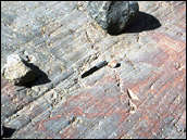
Long parallel grooves on exposed rock faces, called striations, are gouged out by rocks and debris carried on the bottom surface of a flowing glacier. Jean-Pierre Perraudin inferred that striations he saw in valleys far from existing glaciers were caused by glaciers that had since disappeared. (Photograph courtesy Richard S. Williams, Jr., U.S. Geological Survey) | ||

Agassiz quickly developed a broad theory of what he termed the “Ice Age,” a period in which giant glaciers extended down from the North Pole to cover Europe and much of North America. When he presented the theory on July 24, 1837, in a meeting of the Swiss Society of Natural Sciences in Neuchatel, Switzerland, he was met with sheer rage from a scientific community well-established in its views. Agassiz was undeterred. He enthusiastically showed leading scientists evidence of glaciation, and captured the public imagination with his descriptions of an icy Earth. While most scientists disagreed at first, his fervor caught the attention of the community, and by the 1870s, the Ice Age theory was widely accepted. |
Louis Agassiz (1807–1873) found evidence for a past ice age in the mountains of Switzerland. Although controversial at first, his ideas were eventually accepted by the scientific community. Modern scientists have extended his techniques, and developed many new ones, to explore past climates (both warm and cold) in detail. (Drawing courtesy History of Science Collections, University of Oklahoma Libraries.) | ||

| |||
As scientists came to accept that the erratics pointed to an Ice Age, the realization triggered more questions. What had caused the Ice Age, and why had it ended? As fossils of a temperate forest were discovered sandwiched between Ice Age soil layers, scientists’ questions became increasingly more complicated. Could the Ice Ages return? Might our climate change again? Ironically, one of the theories proposed to explain what had caused the Ice Ages to come and go would become the key argument supporting an opposite, and equally controversial, kind of climate change: global warming. In 1895 Svante Arrhenius proposed that the drop in temperatures that occurred during the Ice Age could have been produced by a drop in the concentration of atmospheric carbon dioxide compared to the then-current levels. He even proposed that industrial emissions could raise Earth’s temperature in coming centuries. Despite his theory, most scientists didn’t believe that humans could affect climate until the 1960s, when evidence of human impacts on the natural world were becoming increasingly obvious. Once again, climate change became controversial, as the theory of global warming became one of the biggest scientific debates of the late twentieth century. The questions of the past generation took on a new urgency. Could climate change be a threat to humankind? And could our own actions increase the threat? These questions have compelled scientists to scour the Earth for signs of past climate change. Their search has developed into an entire scientific field: paleoclimatology, the study of past climates. In determining what has triggered climate change in the past, scientists hope to learn how natural and human triggers might change our climate in the future. Most scientists who study the past have fossils and artifacts that help them reconstruct history. But without thermometer readings, how can they know how cold it was when the ice from the last Ice Age began to retreat? Scientists who want to reconstruct past climates gather clues buried in the Earth in much the same way that an archeologist reveals past culture by looking at artifacts or a detective reconstructs a crime scene using multiple bits of evidence. |
Agassiz used detailed drawings of mountainous terrain, glacial erratics, and other glacial features to bolster his theories. The boulder in the left foreground protects the column of ice underneath it from melting, while being carried by the glacier. Eventually, the boulder will be deposited in a moraine, or left behind as an isolated erratic. [Rollover with your cursor to see overlay of features, click to see combined drawing and overlay.] (Drawings adapted from Agassiz) | ||
Climate leaves an imprint on the planet, in the chemical and physical structure of its oceans, life, and land. Some of these artifacts, known as climate proxies, reveal general climate patterns over the entire Earth, while other proxies reveal seasonal change in specific regions. By reading the signs of past climate, scientists reconstructed the history of Earth’s climate over hundreds of thousands—in some cases millions—of years. When combined with observations of Earth’s modern climate into computer models, paleoclimate data help scientists to predict future climate change.
|
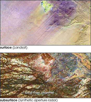
Fossil rivers in the Sahara Desert, now buried by sand, attest to a much wetter climate in the past than now. Only a few faint stream channels are visible in the top image, a false-color scene from Landsat. Radar imagery (lower), which penetrates several meters beneath the sand, reveals a dense network of streambeds. (Images courtesy NASA/JPL imaging radar team) | ||
|
Subscribe to the Earth Observatory About the Earth Observatory Contact Us Privacy Policy and Important Notices Responsible NASA Official: Lorraine A. Remer Webmaster: Goran Halusa We're a part of the Science Mission Directorate |