NPFMC - A Guide to Stock Assessement of Bering Sea & Aleutian Islands Groundfish

David Witherell (North Pacific Fishery Management Council)
& James Ianelli (Alaska Fisheries Science Center, NMFS)

September 1997

North Pacific Fishery Management Council
605 West 4th Avenue, Suite 306
Anchorage, Alaska 99501

How many times have your heard comments like, “Those scientists don't know what they are talking about.” “Stock assessment is a bunch of hocus-pocus,” and “How the heck did those guys come up with those numbers anyway?” The mystery surrounding the stock assessment process has left fishermen, environmentalists, and others with serious questions and concerns about biomass estimates and established harvest rates. In this article, we don’t attempt to teach all there is to know about fish stock assessment (that’s a Ph.D. program and then some!), but wish to provide the layman with a general understanding of how quotas for groundfish in the Bering Sea and Aleutian Islands are established. As a result, we hope to improve communication among fishermen, managers, and scientists.

Stock assessment is essentially a way to estimate how many fish there are and predict how fish populations will respond to harvesting. Assessment scientists use survey and fishery information in mathematical calculations to estimate how many fish are out there (abundance or biomass). Further, information about the life history (growth, maturity, and mortality) of individual fish species is used to estimate how many fish can be caught without impacting future production of young fish. Fishery managers then use the assessment information about biomass and fishing rates to make decisions about the allowable amount of fish that can be caught during the next fishing season. Managers weigh economic and social considerations along with biological advice. Stock assessment scientists, on the other hand, are primarily concerned with biological hunts and variability of stock productions

Assessments of Bering Sea and Aleutian Islands (BSAI) groundfish stocks are prepared by scientists at the National Marine Fisheries Service (NMFS), Alaska Fisheries Science Center (AFSC) in Seattle. The assessments are reviewed annually by the BSAI groundfish plan team which is composed of biologists, economists, and mathematicians from various government agencies and academic institutions. The plan teams compile the individual species assessments into a Stock Assessment and Fishery Evaluation (SAFE) document. The SAFE contains information on historical catch trends, biomass estimates, preliminary estimates of Acceptable Biological Catch (ABC), assessments of harvest impacts, and alternative harvesting strategies. The plan team’srecommendations are then passed on to the Council and it’s advisory committees. To understand the basis for these recommendations, it is necessary to have some basic knowledge of fishery biology and assessment methodology.

Assessing fish stock abundance is not an easy task. You can’t simply count them because the fish are out of sight below the water surface. And counting is further complicated because fish move around. It’s like trying to estimate the number of worms living in the soil in a schoolyard. How would you go about it? Do you dig up all the grass (a Herculean task) in order to physically count each one, or do you conduct a survey by taking a sample shovel-full of soil here and there to get an estimate? For oceanic fish stocks, the survey sampling method is the only feasible option (of course, we don’t use shovels!).

There are several different surveys conducted in the BSAI area, including a bottom trawl survey, a hydoacoustic (sonar type) survey, and longline surveys. Each survey has its strengths and weaknesses for estimating abundance of different fish species. For example, the bottom trawl survey does a good job of estimating rock sole biomass, but does a poorer job with pelagic fishes such as herring and squid. Nevertheless, assessments for most stocks rely on bottom trawl survey data.

The Bering Sea bottom trawl survey is conducted annually during the months of July and August. The survey is based on a grid of fixed survey stations to allow for equal sampling across all habitat types. Each station is located approximately 20 nautical aides apart, giving a sampling intensity of one station for every 1,314 square kilometers (or about 383 square nautical miles). The gear is an Eastern type otter trawl having a 31.4 m longfootrope, and is equipped with a small mesh liner (3.2 cm stretched) to retain juvenile fish and crabs. The catch from each tow is first sorted by species then weighed and counted to come up with total values. Each species component is then sampled for sex determination, lengths, individual weights, and biological samples as needed. Fish scales and otoliths (ear bones used for balance and orientation) may be collected for age and growth information (annual rings are formed on these structures similar to growth rings on a tree stump). Gonads are examined for maturity stage. This information is used to evaluate the reproductive activity of fish at different sizes and age. Stomach samples are also collected to provide food habits data (who’s eating who, and how much?).

Back to top

Current research surveys conducted for Bering Sea and Aleutian Islands groundfish, by species and area.

In the eastern Bering Sea bottom trawl survey, total biomass is estimated using an area-swept method. That is, the length of the net opening multiplied by the distance the net is towed provides a density index for each species at that survey station. The density of fish from all survey stations is averaged and extrapolated to the surveyed area of the Bering Sea to provide a total biomass estimate. Bering Sea bottom trawl survey stations

Survey tows made in areas where a species is not abundant often provide better information about relative stock conditions than samples taken in areas with large aggregations of fish. This is one of the primary reasons why data collected aboard fishing vessels is not exclusively used for estimating biomass; quite simply, fishermen try to fish in areas with the most fish! Also, the same survey gear (whether it be trawl, longline, or sonar) is used at each station year after year. Survey gear is generally designed to catch fish of all sizes, rather than just catching larger fish like the gear used by commercial fishing vessels. Hence, surveys provide a consistent sample of fish from year-to-year, and provide information on pre-recruit sized fish that would otherwise not be available for stock assessment. (Back to top)

Another important source of information comes from commercial fisheries through the observer program. Observers collect size and age data (more otoliths!), in addition to determining total catch of each species. This provides assessment scientists with critical information on removals of fish by age. Commercial samples improve estimates of stock structure and year-class strength (numbers of fish at each age).

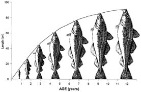
Life history data (particularly growth and maturity data) are also used to determine appropriate harvest rates. Average growth and maturity can be accurately described by equations with parameters developed from these observations, as shown in the figures below. Life history parameters for BSAI groundfish stocks are listed in the adjacent table. From this information, we can calculate length or weight for any age fish.

One of the basic parmeters used in stock assessment calculations is the natural mortality rate, designated as M in equations. Like people and all other living things, a portion of the population dies each year. With good information, we can determine a mortality rate for each age. This forms the basis of life expectancy charts for people by insurance companies. For fish, this is more difficult because the numbers of natural deaths is unobserved for most marine species. Instead, natural mortality is often assumed constant once they reach maturity. To estimate mortality, other life history information is used. For example, we know mortality is related to longevity; when mortality is high, life spans are short. Examination of numerous fish species have provided a general relationship of mortality and longevity (Hoenig’s equation: In (M) = 1.46 - 1.01 * In (t_max)). Because numerous age samples are taken during surveys and commercial fisheries, we have information on longevity that consequently provides us with an estimate of M. For example, if maximum age observed (t_max) for a fish species is 15 years, M = 0.28 based on Hoenig’s formula.

Comparison of annual rate w/instantaneous rates

Assessment scientists use instantaneous rates, rather than percentages, in calculating mortality assuming that mortality occurs throughout the year. This allows mortality due to natural causes (M) and mortality due to fishing (F) to be used together in equations. The instantaneous total mortality rate is denoted as Z; hence F+M=Z. To convert instantaneous rates to annual rates (A), the formula A = l-e^-z, where e is a standard mathematical constant equal to 2.718. A quick chart comparing annual rates with instantaneous rates is shown in the adjacent table. Tiers used to determine ABC & OFL

The primary foundation of fisheries management has been to provide for long-term maximum sustainable yield (MSY) of fish resources. Unfortunately, information has not generally been available to determine the fishing mortality rate that produces MSY, particularly in variable environments. Instead, other surrogate fishing mortality rates have been used. The harvest rate set for each species depends on available information; in general, the less information available, the higher the uncertainty, and the more conservative the harvest rate used (as shown in the adjacent table). Reference fishing mortality rates of F_30% and F_40% are generated when maturity, growth and natural mortality data are available. For most BSAI stocks, our benchmark fishing mortality rates are F_30% to define overfishing, and F_40% to define ABC (tiers 2 through 4). F_40% is the fishing mortality rate that reduces spawning biomass per recruit to 40% of its unfished value. For stocks with very limited information. ABC is based on fishing rates that equal M or just average catches (tiers 5 and 6).

The F_40% exploitation rate was based on analysis of a range of life history parameters and spawner recruit relationships observed for North Pacific and Atlantic groundfish stocks (Clark 1991, 1993). A preliminary analysis indicated that for a range of spawner-recruit relationships, a fishing mortality rate that reduced spawning biomass per recruit to 35% of its unfished value (denoted F_35%) would produce yields of at least 75% of maximum sustainable yield. A subsequent analysis that incorporated recruitment variability suggested that F_40% would be a more conservative fishing rate without reducing long-term yield.

So how do we know the unfished value of a population? As long as we have an estimate of M, average weight at age, and proportion mature at age, we can generate spawner-per-recruit (SPR) reference mortality rates. Calculation of SPR is shown in the table below, by illustrating what happens to 1,000 recruits during their lifetime. In an unfished stock, mortality is due only to “natural” causes (for example predation, starvation, disease). The number of spawners at each age is the product of number alive at age, weight at age, and proportion mature at age. Percent SPR at each age is simply the number of spawners at age divided by the initial number of recruits (1,000 in this example). (Back to top)

Spreadsheet illustrating the calculation of spawner-per-recruit (SPR) in an unfished population and a fished population of Atka mackerel. Calculations begin with 1,000 recruits, reduced over time by natural mortality (M) and fishing mortality (F). Average weight at age (kg) and proportion mature at age comes from direct observations. SPR is the biomass of spawners produced by that age, divided by the number of recruits (1,000). The total for all ages is the SPR for that level of fishing mortality. In this example, we have calculated that F_40% is 0.36.

Unfished Population								Fished Population (F=0.36)
Age	M	F	# of fish	Avg . wt.	Prop. mature	Wt. of Spawn	SPR	Age	M	F	# of fish	Avg . wt.	Prop. mature	Wt. of Spawn	SPR
1 2 3 4 5 6 7 8 9 10 11 12 13 14 15+	0.3 0.3 0.3 0.3 0.3 0.3 0.3 0.3 0.3 0.3 0.3 0.3 0.3 0.3 0.3	0.0 0.0 0.0 0.0 0.0 0.0 0.0 0.0 0.0 0.0 0.0 0.0 0.0 0.0 0.0	1000 741 549 407 301 223 165 122 91 67 50 37 27 20 15	0.23 0.40 0.52 0.59 0.63 0.66 0.68 0.69 0.70 0.70 0.71 0.71 0.71 0.71 0.71	0.00 0.04 0.22 0.69 0.94 0.99 1.00 1.00 1.00 1.00 1.00 1.00 1.00 1.00 1.00	0.0 11.98 62.23 164.49 178.84 145.92 112.25 84.60 63.36 47.26 35.16 26.12 19.39 14.38 10.66.	0.00 0.01 0.06 0.16 0.18 0.15 0.11 0.08 0.06 0.05 0.04 0.03 0.02 0.01 0.01	1 2 3 4 5 6 7 8 9 10 11 12 13 14 15	0.3 0.3 0.3 0.3 0.3 0.3 0.3 0.3 0.3 0.3 0.3 0.3 0.3 0.3 0.3	0 0 0.05 0.25 0.36 0.36 0.36 0.36 0.36 0.36 0.36 0.36 0.36 0.36 0.36	1000 741 522 301 156 80 42 22 11 6 3 2 1 0 0	0.23 0.40 0.52 0.59 0.63 0.66 0.68 0.69 0.70 0.70 0.71 0.71 0.71 0.71 0.71	0.00 0.04 0.22 0.69 0.94 0.99 1.00 1.00 1.00 1.00 1.00 1.00 1.00 1.00 1.00	0.00 11.98 59.19 121.86 92.44 52.62 28.24 14.85 7.76 4.04 2.10 1.09 0.56 0.29 0.15	0.00 0.01 0.06 0.12 0.09 0.05 0.03 0.01 0.01 0.00 0.00 0.00 0.00 0.00 0.00
						Total	1.00							Total	0.40

There are two primary types of assessment methods used for BSAI groundfish, and they are index and age structured models. The most basic assessment is an index of population based on survey data. For an index assessment, biomass is estimated solely from the trawl surveys area-swept extrapolation.

Age structured models include virtual population analysis (VPA) and stock synthesis. An assessment based on VPA use estimates of catch at age data from the fishery to determine the numbers at age. The critical catch at age estimates come from the otolith samples collected by observers during the fisheries. The age samples are then combined with the (typically) large number of length frequency samples and aggregate catch estimates to come up with estimates of the total catch numbers at age. Given these estimates of catch, the total stock biomass and population composition for prior years can thus be determined. The VPA computations simply involve transforming the catch-at-age estimates into historical population estimates through a series of equations. Here, the survey data are typically compared for consistency with results coming from the VPA. If there is poor consistency between the survey and the results from the VPA (or any other “model” for that matter) then the stock assessment scientist must change assumptions made in the VPA or conclude that, given the inherent “noise” from the survey data, the inconsistency is acceptable. The process of changing assumptions typically involves “tuning” population parameter values much like a radio dial is tuned. As the parameter values change, the VPA (or other model) becomes more or less consistent with survey observations.

Reference fishing mortality rates established for Bering Sea and Aleutian Islands groundfish, 1997.

A computer program called “stock synthesis” is used for most BSAI groundfish assessments. This program is fundamentally set up as a tool for easily incorporating complex fishery and survey data in a single framework. It is structured such that it is less demanding than the VPA methods and requires fewer assumptions about the types of data that are entered. By fewer assumptions, we mean that quantities in the model that we know areuncertain are treated appropriately. For example, the foundation of VPA methods requires the assumption that the catch-at-age data are measured without error. The key philosophy of the model is to treat our observations, say the estimates we make on the catch-at-age in a given year, as random quantities about some true underlying values. This simply involves treating the estimation using appropriate statistical methods.

One way to think about how the program is designed is to imagine trying to say something about a stock of fish before looking at any data. What can one do? Well, given that you know the species of fish, and some general biological characteristics, you could synthesize the abundance of that stock given some crude approximation. Given guesses about: (a) how much harvest has been taken over the past several years, (b) the rate these fish grow with age, and (c) how fast they die off due to natural causes. One could come up with a simulated or synthesized level of abundance with this information alone.

Leaving out some details, the essence of our initial data-less or synthesized population model can be illustrated in the following example. First let’s say we think that the fishery had average catches of about 500 tons of catch for the past 10 years (before then removals were insignificant). Then let’s say, we guess that in year 10, the harvest represented about 10% of the total stock. Given some assumptions about the rate fish die due to natural causes (natural mortality) and the average weight at age, the abundance trend can be sketched out (see table below). This result might be completely wrong but the calculations for the construction of population numbers is complete. Now all that is left is to add some realism to this synthesized stock. This is where the data (finally!) comes in.

In our numerical model, we want to replace values describing synthesized stock with numbers that best match our observations. This is analogous to the sculptor chiseling a stone to the desired likeness. First we replace our biological guesses (such as average weights at age) with estimates based on real data. Similarly, we use information on the longevity and reproductive output of the species under consideration to come up with initial estimates of natural mortality rates. Information on the type of gear used in the fishery and surveys provide background on the selectivity patterns we might expect. Running the model at this point improves the realism over our original guesses and scales the population values in general terms. Further refinements occur as age or size composition data are added and provide critical information on the variability of year-class strengths and historical pattern of age structure of the population.

Age	4	5	6	7	8	10+
Natural Mortality Average weight	20% 1.0	20% 1.5	20% 1.9	20% 2.1	20% 2.4	20% 2.6
	Numbers						Biomass	Catch	F
Year 0 (no fishing) Year 1 Year 2 Year 3 Year 4 Year 5 Year 6 Year 7 Year 8 Year 9 Year 10	1,000 1,000 1,000 1,000 1,000 1,000 1,000 1,000 1,000 1,000 1,000	800 737 732 729 725 723 722 720 720 720 720	640 589 539 533 528 524 522 520 518 518 518	512 471 431 393 387 382 378 376 374 373 373	410 377 345 314 285 279 275 272 271 269 269	328 302 276 251 228 206 202 198 196 195 194	6,300 5,900 5,600 5,300 5,200 5,100 5,000 5,000 5,000 5,000 5,000	500 500 500 500 500 500 500 500 500 500	0% 8% 8% 9% 9% 10% 10% 10% 10% 10% 10%

These refinements reveal the great utility of computers in the final estimation process. For example, we could enter a model into a spreadsheet and manipulate a few key values until the “model” fit our observations. With several hundred parameters, however, doing this by hand is impractical so specialized automatic “tuners” to do the model fitting. This simply changes parameter values until our “simulation” becomes most consistent with our observations. Tuning computer models is also called optimization. Optimization is an active area of computer science research and is applied for solving a wide variety of problems from business decisions to analyses of quantum mechanics. In our fisheries applications, we attempt to take advantage of these rapid technological developments to help improve our ability to provide useful advice to fisheries managers. These steps are incremental and, as with other sciences, hotly debated and always evolving.

One concern about how fisheries stock assessments can fail is in providing harvest guidelines without consideration of how robust or resilient a model result is to harvest recommendations. Dealing with uncertainty is an extremely difficult task. In most stock assessments around the world, the magnitude of the uncertainty (if this is presented at all) is probably largely underestimated. Terms like precautionary principle and risk averse policy are becoming increasingly common and for good reason. These terms are most applicable where effective management practices are in place (e.g., quotas in the North Pacific). The amount of precaution and risk aversion recommended based on stock assessment analyses is irrelevant if there are no means to control the level of fishing, The idea of risk aversion is problematic since the concept of risk is different for different people or fisheries sectors. For example, most commercially exploited species of fish are unlikely to face the risk of extinction sinceeconomic factors will be generally prohibitive to catching the very last fish. There are real risks of economic collapses of fisheries or ecosystem imbalances caused by fisheries. Studies on ecosystems is difficult since there are so many factors involved, prediction is probably more difficult than predicting the weather. Recent advances that have been made (and we currently part of the quota tier system presented above) reflect the fact that when there is greater uncertainty about key quantities, the risk averse policy generally results in lower quotas. Fisheries scientists enjoy this result since the need for better information can translate to more accurate understanding of fish population dynamics while providing a real service to the management of these fisheries. (The Precautionary Principle in North Pacific Groundfish Management, by Dr. G. Thompson (AFSC NMFS, Seattle, WA). Available at: http://www.refm.noaa.gov/grant/precaut.html.)

The stock assessment results and projections for 1997 were summarized in the SAFE document released in November 1996. The SSC reviewed the SAFE, and for many species, concurred with the plan team’s estimate of biomass and recommended harvest rates. For Bogoslof pollock, the SSC disagreed with the team, and recommended that the OFL and ABC be reduced by current biomass. A similar adjustment was recommended for Greenland turbot. The Council’s Advisory Panel recommended the total allowable catches (TACs) for 1997, which were adopted by the Council. In all cases, TAC is less than or equal to ABC that is less than OFL. The 1997 specifications are shown in Appendix Table 2 at right.

Back to top OR

Species	Area	EBS Trawl Survey 1979-	EBS Acoustic Survey 1979-	Bogoslof Acoustic Survey 1988	EBS+AI Longline Survey 1996-	AI Trawl Survey 1980-
Pollock Pacific cod Yellowfin sole Gr. turbot Arrowtooth Rock sole Flathead sole Other flatfish Sablefish P. ocean perch Sharp/Northern Short/Rougheye O. red rockfish Other rockfish Atka mackerel Squid Other species	BS AI Bogoslof BSAI BSAI BSAI BSAI BSAI BSAI BSAI BS AI BS AI AI AI BS BS AI AI BSAI BSAI	annual - - annual annual annual annual annual annual annual annual - annual - - - annual annual - - annual annual	triennial - - - - - - - - - - - - - - - - - - - - -	- - annual - - - - - - - - - - - - - - - - - - -	- - - - - - - - - - biennial biennial - - - - - - - - - -	- triennial - - - - - - - - - triennial - triennial triennial triennial - - triennial triennial - -